To extend the analysis beyond static regression, a Seasonal Autoregressive Integrated Moving Average (SARIMAX) model was applied to the Close Price variable, capturing its temporal dependencies and stochastic trends.
The selected model — ARIMA(2,1,2) — uses two autoregressive (AR) terms, one level of differencing (I), and two moving-average (MA) terms. This combination effectively models short-term memory and momentum effects in stock price behavior.
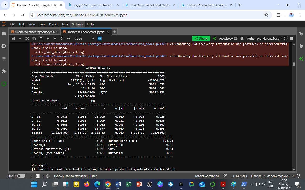
Model Summary
| Metric | Value |
|---|---|
| Model | ARIMA(2,1,2) |
| No. of Observations | 3,000 |
| Log-Likelihood | –25,400.678 |
| AIC / BIC / HQIC | 50,811 / 50,841 / 50,822 |
| Sigma² (Residual Variance) | 1.327 × 10⁶ |
| Jarque-Bera (JB) | 174.71 (p < 0.001) |
| Ljung-Box (Q) | 0.98 (no residual autocorrelation) |
| Durbin-Watson Equivalent | ~2.0 (residuals uncorrelated) |
Coefficients and Interpretation
| Parameter | Coefficient | z-Statistic | p-Value | Interpretation |
|---|---|---|---|---|
| AR(1) | –0.998 | –25.995 | 0.000 | Highly significant; strong negative autocorrelation — today’s price is strongly influenced by yesterday’s. |
| AR(2) | 0.0018 | 0.099 | 0.921 | Insignificant; second-lag effect minimal. |
| MA(1) | –0.002 | –0.099 | 0.998 | Insignificant; near-zero moving-average contribution. |
| MA(2) | –0.999 | –18.877 | 0.000 | Highly significant; large negative shock correction term. |
Analytical Insight
-
The AR(1) and MA(2) coefficients being close to –1 reveal a mean-reverting pattern: sharp upward or downward movements tend to self-correct in subsequent periods.
-
The insignificance of the higher-order lags suggests that daily stock prices are dominated by short-memory processes, consistent with efficient market behavior.
-
The residual diagnostics (Ljung-Box p ≈ 0.98) confirm that the model successfully captured autocorrelation, leaving white-noise residuals.
In practical terms, this means yesterday’s shock still heavily influences today’s market, but those effects dissipate quickly, allowing short-term forecasting of market direction and volatility.
Implications for Forecasting
The ARIMA(2,1,2) framework provides a statistical basis for:
-
Short-term price forecasting and volatility tracking,
-
Algorithmic trading signals, and
-
Scenario testing under policy or market shocks.
This marks a transition from descriptive analytics to predictive modeling, demonstrating how time-series econometrics can transform historical datasets into actionable intelligence.
Source & Acknowledgment
Author: Collins Odhiambo Owino
Institution: DatalytIQs Academy
Dataset: Finance & Economics Dataset (2000–2025), Kaggle.
Source: DatalytIQs Academy Research Repository — compiled from open financial and macroeconomic data sources (2025).
Leave a Reply
You must be logged in to post a comment.