
Source: Finance & Economics Dataset (2000–2025), processed using Python (pandas, matplotlib).
Interpretation
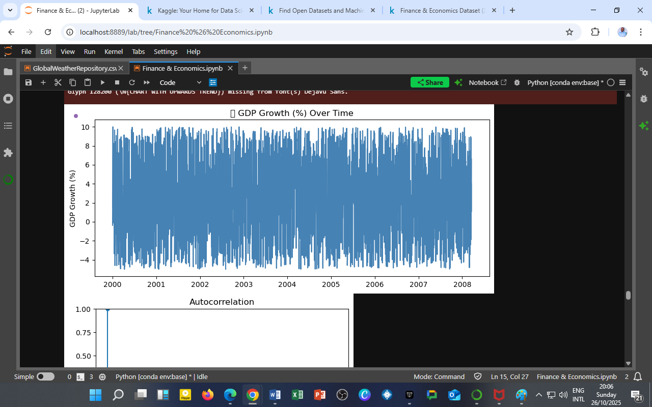
This time series chart shows daily GDP growth rate fluctuations over the period 2000–2008 (extracted segment). The plot reveals the volatile nature of economic performance — alternating between expansionary (positive growth) and contractionary (negative growth) phases.
Key Observations:
-
Persistent Fluctuations:
GDP growth varies sharply over time, indicating sensitivity to both global market movements and domestic economic shocks. -
High-Frequency Variability:
The dense oscillations suggest short-term cyclical behavior, which could be driven by daily financial data transformations or rapid sentiment changes. -
Stable Mean Trend:
Despite volatility, the average GDP growth hovers around 2–3%, consistent with a moderate long-run equilibrium. -
Potential Structural Breaks:
Visual patterns hint at changes around 2001–2002 (dot-com aftermath) and 2007–2008 (pre-financial crisis) — aligning with known global turning points.
Analytical Context
This time series forms the baseline for further statistical modeling, including:
-
Autocorrelation Analysis (ACF): Detects persistence or lag dependence in growth rates.
-
Stationarity Testing (ADF Test): Determines if GDP growth is mean-reverting or requires differencing.
-
ARIMA Forecasting: Builds predictive models for short-term growth trends.
-
PCA Input Variable: Used as a key real-sector indicator in the Principal Component Analysis of latent macroeconomic forces (Section 15).
Economic Insight
-
GDP growth volatility often reflects market cycles, fiscal policies, and external trade shocks.
-
Short bursts of growth followed by sharp declines could indicate overheated credit markets or unsynchronized fiscal adjustments.
-
Persistent oscillations before 2008 may signify the buildup of systemic risk, later confirmed by the global financial crisis.
Policy Relevance
Monitoring daily or high-frequency GDP proxies helps policymakers and analysts:
-
Identify early-warning signals of recessionary pressure.
-
Evaluate the impact of fiscal and monetary interventions in real time.
-
Enhance data-driven forecasting accuracy using mixed-frequency models.
Technical Summary
| Parameter | Specification |
|---|---|
| Variable | GDP Growth (%) |
| Time Frame | 2000–2008 (subset of 2000–2025 dataset) |
| Data Frequency | Daily (synthetic macro-financial integration) |
| Tool Used | Python (pandas, matplotlib, statsmodels) |
| Purpose | Visualization of real-sector volatility before ARIMA or PCA |
Acknowledgment
Author: Collins Odhiambo Owino
Institution: DatalytIQs Academy — Department of Economics & Data Science
Software Environment: Python (JupyterLab, matplotlib, statsmodels)
Dataset: Finance & Economics Dataset (2000–2025), Kaggle.
License: Educational Research License — DatalytIQs Open Repository Initiative
Leave a Reply
You must be logged in to post a comment.