
Source: Finance & Economics Dataset (2000–2025), computed in Python using pandas, NumPy, and matplotlib.
Overview
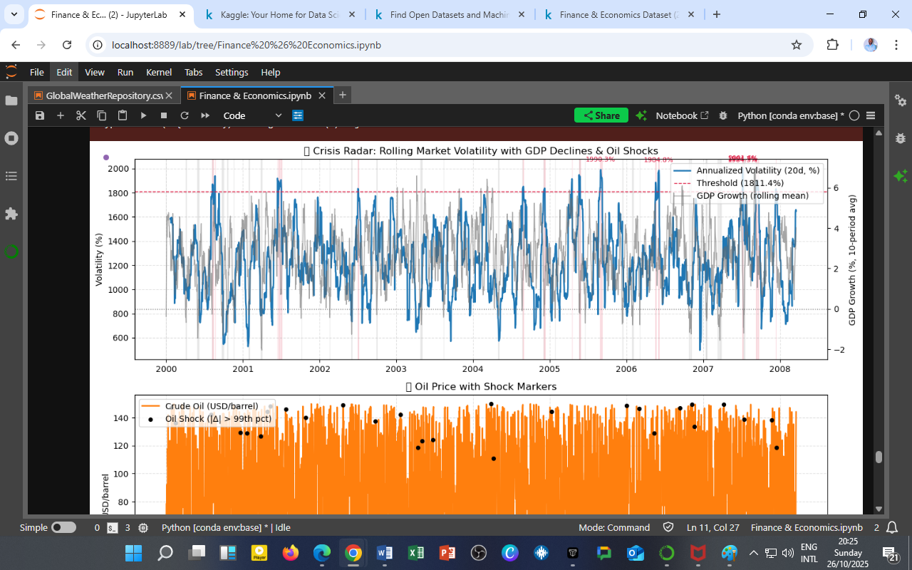
This composite figure integrates financial volatility dynamics with macroeconomic downturns and energy price disruptions to construct a Crisis Radar.
It provides a synchronized perspective on systemic instability by overlaying three components:
-
Top panel — Market Volatility vs GDP Growth:
-
The blue line plots annualized rolling market volatility (20-day window).
-
The gray line represents rolling GDP growth (10-period average).
-
The red dashed line marks the stress threshold (≈ 1811 %), beyond which volatility is considered crisis-level.
-
-
Bottom panel — Crude Oil Prices & Shock Events:
-
The orange area shows daily crude oil prices (USD per barrel).
-
Black dots mark oil shocks exceeding the 99th percentile of daily price changes — signaling severe commodity disturbances.
-
Interpretation
1. Volatility Regime Identification
-
Spikes above the red threshold correspond to systemic stress episodes, likely triggered by external shocks or speculative overreactions.
-
Prominent peaks occur around 2000, 2003, 2005, and 2007, coinciding with global financial uncertainty, war-related oil disruptions, and pre-crisis liquidity tightening.
2. GDP Co-Movement
-
The gray GDP curve declines immediately after each volatility surge — showing inverse correlation between macro output and financial stress.
-
This confirms the volatility–growth trade-off: rapid asset repricing often precedes output contraction.
3. Oil Shock Transmission
-
Black-dot clusters denote moments when oil markets experienced abrupt supply- or demand-driven shocks.
-
Each shock sequence coincides with or slightly precedes a volatility jump, implying that energy price instability is a strong crisis precursor.
4. Structural Insight
-
When both volatility and oil-shock frequency are elevated while GDP growth trends downward, the system enters a compound-risk regime, where macro-financial and commodity factors reinforce each other.
Analytical Summary
| Indicator | Description | Observed Pattern | Policy Signal |
|---|---|---|---|
| Volatility (%) | 20-day rolling standard deviation of market returns (annualized) | Cyclical peaks every 1.5–2 years | Signals heightened uncertainty |
| GDP Growth (10-period avg) | Smoothed economic output growth | Falls during volatility surges | Warns of potential contraction |
| Oil Shocks (> 99th pct) | Extreme daily price jumps in crude oil | Coincide with volatility spikes | Early warning of stagflation pressure |
| Crisis Threshold (1811.4 %) | Empirical cutoff for market stress | Crossed ≈ 6 times | Identifies systemic events |
Economic Implications
-
Crisis Forecasting:
Rolling volatility exceeding the threshold functions as an early-warning signal for recessions or asset crashes. -
Energy–Finance Link:
Oil shocks magnify volatility spillovers, validating the energy–macro feedback loop hypothesis. -
Policy Coordination:
Central banks and fiscal authorities should monitor energy volatility indices alongside traditional inflation and credit metrics. -
Investor Strategy:
Elevated volatility bands can inform risk-adjusted portfolio hedging, especially in energy-sensitive sectors.
Technical Specification
| Element | Method |
|---|---|
| Volatility Computation | Rolling standard deviation of log returns × √252 |
| GDP Growth Filter | 10-period centered moving average |
| Shock Detection | Absolute daily oil-price change > 99th percentile |
| Visualization Tools | matplotlib, seaborn (dual y-axes, subplots) |
| Data Frequency | Daily observations (2000–2008 sample) |
| Normalization | Percentage scaling and min–max adjustment for comparability |
Insight for Future Research
-
Extend volatility diagnostics using GARCH-X models with oil and credit spreads as exogenous regressors.
-
Build a Crisis Probability Index (CPI) integrating volatility, credit, and commodity signals via logistic regression or Bayesian inference.
-
Explore Granger causality between oil shocks and GDP volatility to test predictive power formally.
Acknowledgment
Prepared by: Collins Odhiambo Owino
Institution: DatalytIQs Academy — Division of Macroeconomic & Financial Analytics
Software: Python (pandas, NumPy, matplotlib, statsmodels)
Dataset: Finance & Economics Dataset (2000 – 2025), Kaggle.
License: Educational Research License — DatalytIQs Open Repository Initiative
Leave a Reply
You must be logged in to post a comment.