The Pulse of a Planetary System
Every planet tells time — not with hours, but with orbits.
The orbital period (how long a planet takes to complete one revolution around its star) defines its temperature, atmospheric chemistry, and habitability potential.
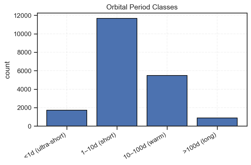
To see how Kepler’s planets compare, we classified them into four period ranges and plotted their counts.

What the Distribution Shows
| Period Range | Label | Interpretation |
|---|---|---|
| < 1 day | Ultra-short-period planets | Rare worlds orbiting extremely close to their stars. These are often rocky and tidally locked, with blistering temperatures. |
| 1–10 days | Short-period planets | The most common classes — “hot Jupiters” and “warm Neptunes” that transit frequently and are easiest to detect. |
| 10–100 days | Warm-period planets | Moderately spaced systems that might include potentially habitable super-Earths. |
| > 100 days | Long-period planets | Rare detections — they require years of observation to confirm transits. These likely represent the colder outer worlds of their systems. |
The sharp peak at 1–10 days highlights how detection efficiency shapes our understanding: Kepler found mostly close-orbiting planets because they transit their stars more often, making them easier to confirm.
In contrast, the long-period tail reflects both astrophysical rarity and observational bias — Kepler’s mission duration simply wasn’t long enough to repeatedly capture their transits.
Connecting the Dots
This distribution reinforces key lessons from your earlier analyses:
| Earlier Finding | Reinforced Insight |
|---|---|
Random Forest importance of log_period |
Confirms period’s predictive power — it strongly affects both cluster formation and detectability. |
| Clustering results (k = 3) | Suggests distinct groups of exoplanets tied to their orbital spacing. |
| Sky map density | The same regions rich in short-period detections are visible in the Mollweide projection — showing Kepler’s observational footprint. |
Together, these plots tell a cohesive story:
The way we see exoplanets depends on how often they cross their stars — and how long we’ve been watching.
Policy and Research Implications
| Focus Area | Recommendation | Impact |
|---|---|---|
| Observation Strategy | Design future telescopes to sustain longer missions (10+ years). | Captures long-period planets similar to Jupiter or Saturn. |
| Data Integration | Combine Kepler, TESS, and JWST datasets for period completeness. | Builds holistic planetary catalogs beyond short orbits. |
| Machine Learning Training | Use balanced datasets or simulated long-period samples. | Reduces bias in AI-based exoplanet detection pipelines. |
| Open Science Policy | Mandate accessible metadata on orbital uncertainty and duration. | Promotes fairness and transparency in exoplanet classification. |
Acknowledgements
-
Dataset: NASA Kepler Exoplanet Archive (via Kaggle).
-
Analysis: Collins Odhiambo Owino — Lead Data Scientist, DatalytIQs Academy.
-
Tools: Python (
matplotlib,pandas,seaborn). -
Institutional Credit: DatalytIQs Academy — transforming astronomical data into scientific insight and educational value.
Closing Reflection
“Planets dance to their stars’ rhythm — and our telescopes catch only those who spin fast enough.”
Understanding orbital period classes reminds us that the universe is vast not only in space but in time.
The next generation of missions — and data scientists — will need patience, precision, and policy vision to hear the full cosmic rhythm.
Leave a Reply
You must be logged in to post a comment.