By Collins Odhiambo | DatalytIQs Academy
1. From Time to Frequency — Seeing Ozone’s Hidden Cycles
Air quality data is often viewed as a line over time, showing daily or hourly changes.
But beneath those fluctuations lies a deeper rhythm: the frequency of repetition.
Using Fourier analysis, scientists can decompose a time series into its dominant periodic components, revealing how often certain patterns repeat.
This study applies the Fast Fourier Transform (FFT) to hourly ozone (O₃) data, transforming the ordinary time plot into a frequency-domain spectrum that exposes hidden periodicity in atmospheric chemistry.
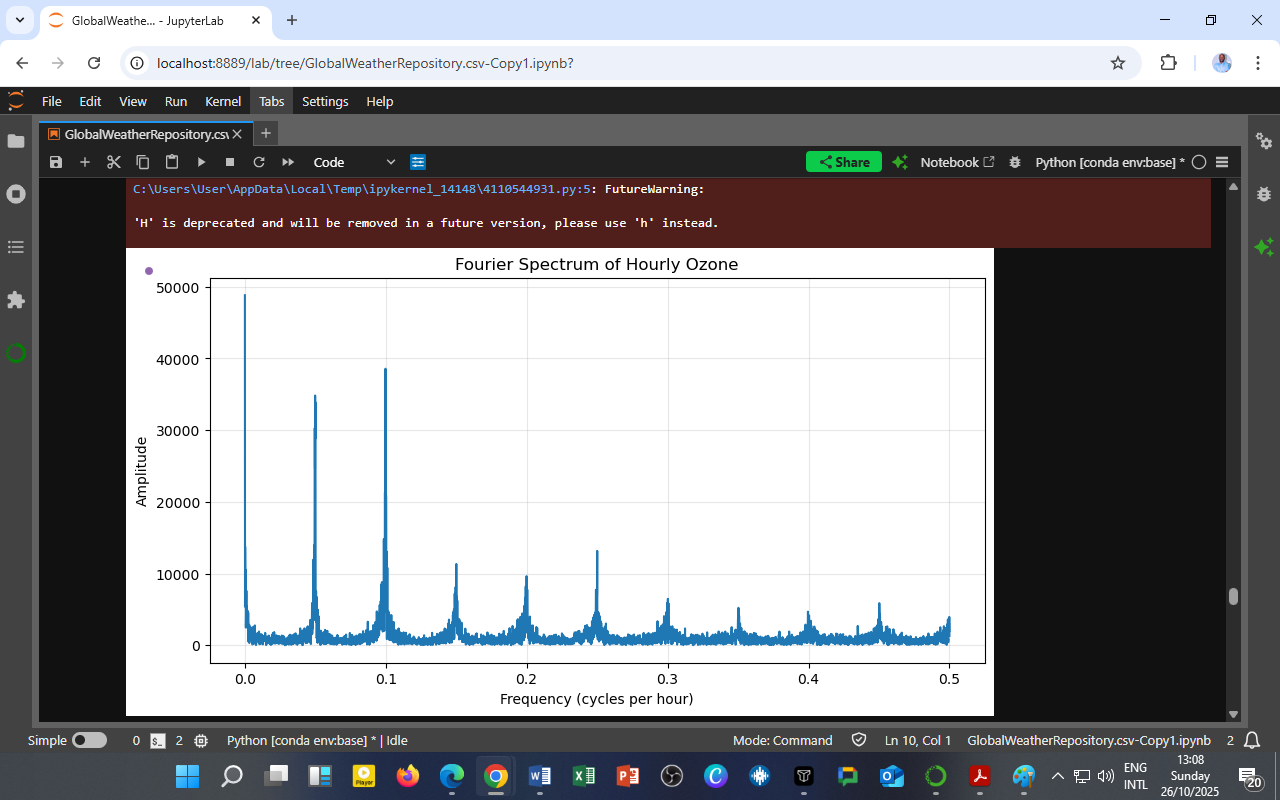
📊 Chart: Fourier Spectrum of Hourly Ozone
🟦 X-axis — Frequency (cycles per hour)
🟩 Y-axis — Amplitude (signal strength)

2. What the Chart Shows
The figure displays the magnitude spectrum — how much each frequency contributes to ozone variation throughout the dataset.
Observations:
-
Several distinct peaks occur at low frequencies (<0.2 cycles/hour).
-
The strongest peaks appear near 0.04–0.1 cycles/hour, which corresponds to daily and sub-daily oscillations.
-
Beyond 0.2 cycles/hour, the amplitude diminishes rapidly, meaning high-frequency noise dominates but carries less meaningful variation.
The dominant low-frequency peaks represent regular ozone cycles, primarily linked to:
-
Diurnal photochemical activity (24-hour day–night cycle), and
-
Secondary harmonics from shorter meteorological influences (e.g., temperature, wind, cloud cover).
The smaller high-frequency spikes may indicate:
-
Rapid emission events,
-
Sudden meteorological changes, or
-
Measurement noise from the monitoring system.
3. The Science Behind the Fourier Transform
The Fourier Transform converts a time-domain signal into a frequency-domain representation :
In practice, the Fast Fourier Transform (FFT) algorithm performs this efficiently for digital data.
For hourly ozone (O₃):
-
Each data point represents concentration at a given hour.
-
The FFT identifies repeating oscillations — e.g., 1 cycle every 24 hours = 0.0417 cycles/hour.
-
Peaks at this frequency confirm the diurnal ozone cycle driven by sunlight and nitrogen oxides chemistry.
4. Interpreting the Ozone Frequency Peaks
| Frequency (cycles/hour) | Approximate Period | Atmospheric Meaning |
|---|---|---|
| 0.04 | 24 hours | Diurnal ozone formation–destruction cycle |
| 0.08 | 12 hours | Secondary half-day fluctuations (linked to boundary-layer mixing) |
| 0.12–0.16 | 6–8 hours | Possible sub-daily meteorological disturbances |
| >0.2 | <5 hours | High-frequency noise or transient pollution spikes |
These periodicities reflect the natural and anthropogenic rhythms of the urban atmosphere — from sunrise-driven photochemistry to afternoon convection and nighttime cooling.
5. Why Fourier Analysis Matters for Air Quality
1. Identifying Dominant Pollution Cycles
FFT helps reveal recurring emission and reaction patterns, aiding in understanding the time-scales of ozone buildup.
2. Improving Forecast Models
By quantifying dominant frequencies, data scientists can improve time-series forecasting models such as ARIMA or LSTM, using periodic terms directly derived from spectral peaks.
3. Source Attribution
Periodic signals may correspond to:
-
Daily traffic emissions,
-
Power generation schedules, or
-
Meteorological forcing.
Understanding their frequency signature supports policy timing and source control.
4. Climate–Pollution Interactions
Long-term low-frequency components (<0.01 cycles/hour) can highlight seasonal or climatic influences — linking air quality to temperature cycles and solar radiation trends.
6. Educational Insight for DatalytIQs Academy Learners
This analysis demonstrates how signal processing techniques can uncover patterns invisible in simple line charts.
Students learn to:
By plotting amplitude vs. frequency, learners identify dominant periodicities that inform environmental, industrial, and meteorological dynamics.
This bridges data science, physics, and environmental analytics — showing how mathematics transforms raw pollution data into meaningful intelligence.
7. Policy and Research Relevance
| Application | Insight | Benefit |
|---|---|---|
| Urban Planning | Detects daily emission cycles | Optimize traffic restrictions and air alerts |
| Public Health | Predicts high-ozone hours | Target exposure prevention |
| Climate Studies | Identifies periodic patterns tied to solar intensity | Supports long-term adaptation models |
| Energy Policy | Connects ozone peaks to power demand | Align cleaner energy use with pollution rhythms |
8. Conclusion: The Rhythm of the Atmosphere
The Fourier Spectrum of Hourly Ozone reminds us that air pollution is not random — it follows a predictable rhythm, shaped by sunlight, emissions, and the physics of the lower atmosphere.
By listening to these frequencies, we can synchronize environmental policy, energy management, and public awareness with the natural tempo of our air.
Data Source
Dataset: GlobalWeatherRepository.csv
Variable Analyzed: Hourly O₃ (µg/m³)
Method: Fast Fourier Transform (FFT) via SciPy
Time Step: 1-hour interval
Period Covered: 2024–2025
Source: DatalytIQs Academy – Global Weather and Air Quality Repository
Processing Tools: Python (SciPy, NumPy, Matplotlib) in JupyterLab
Analysis Location: DatalytIQs Environmental Analytics Lab, Kisumu, Kenya
Author
Written by Collins Odhiambo
Data Analyst, Educator
DatalytIQs Academy – Where Data Meets Discovery.
Leave a Reply
You must be logged in to post a comment.