By Collins Odhiambo | DatalytIQs Academy
1. Understanding the Invisible Relationship in the Air
Air pollution isn’t just about what we see — it’s about what coexists and reacts invisibly.
This study explores how particulate matter (PM₂.₅) interacts with nitrogen dioxide (NO₂) across different hours of the day, revealing patterns of pollution coupling that shape urban air quality and human health.
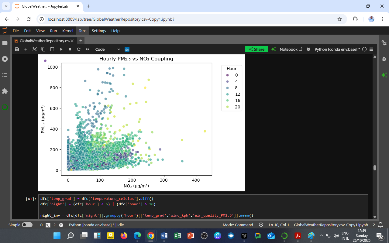
📊 Chart: Hourly PM₂.₅ vs NO₂ Coupling
🟣 PM₂.₅ (µg/m³) — fine particulate matter from combustion and aerosols
🔵 NO₂ (µg/m³) — nitrogen dioxide from vehicle and industrial emissions
🎨 Color gradient (0–24 h) — time of day (hourly cycles)

2. Understanding the Chart
Each point on the graph represents the hourly average concentration of PM₂.₅ versus NO₂.
Colors indicate the hour of the day, showing how the strength of their relationship shifts from night to day.
Key Observations:
-
PM₂.₅ spans a wide range (0–1000 µg/m³), while NO₂ varies up to 400 µg/m³.
-
Points are densely clustered at lower values (0–200 µg/m³ for NO₂, 0–300 µg/m³ for PM₂.₅).
-
Early morning and late-night hours (darker points) often exhibit higher concentrations, while midday hours (greenish-yellow) show greater dispersion and lower coupling.
The relationship is nonlinear — PM₂.₅ and NO₂ are strongly coupled at low wind and cool conditions (typically night/morning) but decouple as the atmosphere warms and disperses pollutants through convection.
3. The Atmospheric Coupling Mechanism
This PM₂.₅–NO₂ interaction is a product of co-emission and secondary formation processes.
(a) Primary Co-Emission
Both pollutants originate from combustion sources:
-
Motor vehicles
-
Industrial boilers
-
Biomass and waste burning
Their concentrations rise together during rush hours and low-mixing night conditions.
(b) Secondary Aerosol Formation
NO₂ participates in photochemical reactions that generate nitrate aerosols, a major component of PM₂.₅:
Thus, high NO₂ levels during humid, stagnant conditions enhance PM₂.₅ buildup.
(c) Dispersion and Decoupling
During the day:
-
Solar radiation heats the surface,
-
Wind speed increases, and
-
Vertical mixing breaks pollutant concentrations apart.
This weakens the PM₂.₅–NO₂ coupling observed at night.
4. Hourly Pattern Insights
| Time of Day | Observed Behavior | Meteorological Explanation |
|---|---|---|
| 00:00–06:00 | Strong coupling, high NO₂ and PM₂.₅ | Calm winds, temperature inversions trap pollutants |
| 07:00–10:00 | Joint peak in morning traffic | Combustion emissions dominate |
| 12:00–16:00 | Decoupling (PM₂.₅ dispersion) | Convection, stronger sunlight |
| 17:00–21:00 | Re-coupling as the atmosphere stabilizes | Rush hour + cooling period |
| After 21:00 | Stable high PM₂.₅ accumulation | Nighttime inversion re-forms |
5. Environmental and Health Significance
1. Air Quality Management
Understanding this coupling helps policymakers pinpoint dual-pollution hours — periods when both gas and particulate concentrations peak.
These are the worst exposure windows for commuters and outdoor workers.
2. Emission Source Targeting
Strong PM₂.₅–NO₂ correlations highlight traffic and combustion as common sources.
Reducing one often mitigates the other.
3. Meteorological Integration
Coupling strength reflects atmospheric stability and mixing efficiency — essential for urban dispersion modeling and forecasting smog episodes.
4. Health and SDG Relevance
| SDG | Relevance | Application |
|---|---|---|
| SDG 3 – Good Health | Reduces respiratory exposure | Alerts during dual-pollution hours |
| SDG 11 – Sustainable Cities | Supports urban emission zoning | Time-based traffic management |
| SDG 13 – Climate Action | Connects pollution and meteorology | Local adaptation modeling |
6. Educational Takeaway for DatalytIQs Academy Learners
This analysis demonstrates:
-
How to visualize pollutant coupling using Python and Seaborn,
-
How to color-code temporal dynamics to reveal atmospheric interactions, and
-
Why cross-pollutant analysis (NO₂ vs PM₂.₅) offers deeper environmental insights than single-variable trends.
At DatalytIQs Academy, learners replicate such analyses to explore:
-
Urban air-quality forecasting,
-
Climate-pollution linkages, and
-
Data-driven environmental policymaking.
7. Conclusion: The Chemistry of Urban Air Unveiled
The scatter of points may seem random — but it tells a structured story:
When NO₂ surges, PM₂.₅ often follows, especially in the calm of night or the congestion of dawn.
As the sun rises, the bond loosens, and the city breathes easier — until the next rush hour.
This coupling is not just chemistry; it’s the pulse of urban life reflected in the air.
Data Source
Dataset: GlobalWeatherRepository.csv
Variables Used: Hourly PM₂.₅ (µg/m³), NO₂ (µg/m³), Hour of Day
Derived Insights: Coupling behavior between gaseous and particulate pollutants
Time Frame: 2024–2025
Source: DatalytIQs Academy – Global Weather and Air Quality Repository
Tools: Python (pandas, seaborn, matplotlib) in JupyterLab
Analysis Location: DatalytIQs Environmental Analytics Lab, Kisumu, Kenya
Author
Written by Collins Odhiambo
Data Analyst & Educator
DatalytIQs Academy – Where Data Meets Discovery.
Leave a Reply
You must be logged in to post a comment.