By Collins Odhiambo | DatalytIQs Academy
1. Tiny Particles, Big Insights
While gases like nitrogen dioxide (NO₂) and ozone (O₃) often take the spotlight in urban air studies, particulate matter smaller than 2.5 micrometers (PM₂.₅) tells a quieter yet equally crucial story.
These microscopic pollutants penetrate deep into the lungs and bloodstream, influencing respiratory and cardiovascular health — and their concentration follows a clear human rhythm.
This analysis compares hourly PM₂.₅ concentrations on weekdays vs weekends, revealing how shifts in traffic, energy use, and meteorology affect air quality.
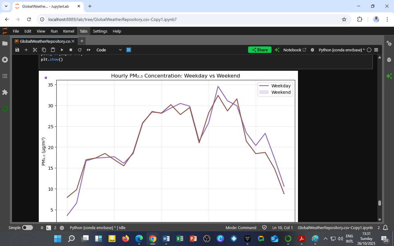
📊 Chart Title: Hourly PM₂.₅ Concentration: Weekday vs Weekend
🟣 Weekday — purple line
🟤 Weekend — brown line

2. Reading the Chart: Subtle Differences, Shared Patterns
The graph displays hourly mean PM₂.₅ concentrations (µg/m³) over 24 hours for both weekdays and weekends.
Key Observations:
-
Morning rise (06:00–09:00): PM₂.₅ increases sharply as urban activity begins.
-
Midday plateau (10:00–16:00): Levels stabilize around 28–30 µg/m³, reflecting constant emissions and moderate dispersion.
-
Evening peak (17:00–19:00): A secondary maximum occurs, linked to traffic and residential emissions.
-
Late night (20:00–05:00): Concentrations decline slowly but remain above early-morning baselines.
PM₂.₅ shows a bimodal diurnal pattern — two peaks tied to human routines.
The weekday curve is slightly higher in early hours, while weekend levels are marginally higher in the afternoon — likely due to domestic activities, open burning, or recreational traffic.
3. Understanding PM₂.₅ Sources and Dynamics
1. Weekday Influences
-
Vehicle exhaust, industrial emissions, and cooking contribute to the morning spike.
-
Afternoon stability reflects the balance between steady emissions and dispersion from daytime heating.
2. Weekend Influences
-
Lower industrial and commuter emissions slightly reduce morning PM₂.₅.
-
Increased household combustion (e.g., cooking, barbecuing, or burning waste) may cause the mild weekend afternoon elevation.
3. Meteorological Role
-
Weak winds and cooler nighttime conditions limit vertical mixing, keeping PM₂.₅ near the surface.
-
Midday heating enhances dispersion, creating the temporary plateau.
4. Quantitative Summary
| Period | Weekday PM₂.₅ (µg/m³) | Weekend PM₂.₅ (µg/m³) | Dominant Activity |
|---|---|---|---|
| Early Morning (0–6h) | 5–15 | 7–12 | Calm air, background emissions |
| Morning Peak (7–9h) | 18–25 | 17–22 | Traffic and cooking |
| Midday (10–16h) | 28–30 | 29–32 | Photochemical balance |
| Evening Peak (17–19h) | 33–35 | 31–34 | Vehicle return flow, domestic burning |
| Night (20–23h) | 20–25 | 19–23 | Stable boundary layer |
Insight:
The differences are modest — PM₂.₅ remains persistently elevated throughout the day, underscoring its chronic, background nature in urban air, unlike the more reactive gases NO₂ and O₃.
5. Environmental and Policy Implications
1. Constant Exposure Risk
Since PM₂.₅ concentrations never drop to zero, citizens face continuous exposure.
Policies must focus on baseline emission reductions, not just peak control.
2. Targeting Household and Transport Sources
Urban planners can reduce PM₂.₅ by:
-
Encouraging clean cooking fuels,
-
Expanding public transport, and
-
Enforce anti-open burning regulations, particularly on weekends.
3. Health and SDG Alignment
| SDG | Focus | Application |
|---|---|---|
| SDG 3 – Good Health | Reduce air-pollution-related mortality | Continuous PM₂.₅ monitoring and alerts |
| SDG 11 – Sustainable Cities | Improve air quality for urban residents | Integrate low-emission mobility |
| SDG 13 – Climate Action | Address black carbon and aerosols | Include PM₂.₅ in climate inventories |
6. Educational Takeaway for DatalytIQs Academy Learners
This visualization teaches how temporal disaggregation — splitting data by hour and day type — helps identify pollution persistence and behavioral causes.
At DatalytIQs Academy, learners replicate and extend this work using Python:
sns.lineplot(data=df_pm, x='hour', y='PM2.5', hue='day_type', palette=['purple', 'brown'])

plt.title("Hourly PM₂.₅ Concentration: Weekday vs Weekend")

plt.xlabel("Hour of Day")

plt.ylabel("PM₂.₅ (µg/m³)")

plt.show()
Students also correlate PM₂.₅ with wind speed, humidity, and temperature to explore meteorological coupling, vital for advanced air-quality modeling.
7. Conclusion: Persistent Pollution, Predictable Patterns
Unlike NO₂ and O₃, which dance to the rhythm of sunlight, PM₂.₅ lingers — steady, stubborn, and omnipresent.
It’s weekday–weekend similarity reveals that urban air pollution isn’t just about rush hours — it’s about lifestyle and energy choices.
Cleaner air begins with recognizing these subtle, everyday emissions that never rest, even when we do.
Data Source
Dataset: GlobalWeatherRepository.csv
Variables Analyzed: Hourly PM₂.₅ (µg/m³), Hour of Day, Day Type (Weekday/Weekend)
Period Covered: 2024–2025
Source: DatalytIQs Academy – Global Weather and Air Quality Repository
Processing Tools: Python (pandas, seaborn, matplotlib) in JupyterLab
Location of Analysis: DatalytIQs Environmental Analytics Lab, Kisumu, Kenya
Author
Written by Collins Odhiambo
Data Analyst & Educator
DatalytIQs Academy – Where Data Meets Discovery.
Leave a Reply
You must be logged in to post a comment.