Blog

  • BMW Annual Sales Trends by Fuel Type (2010–2024)

    Overview

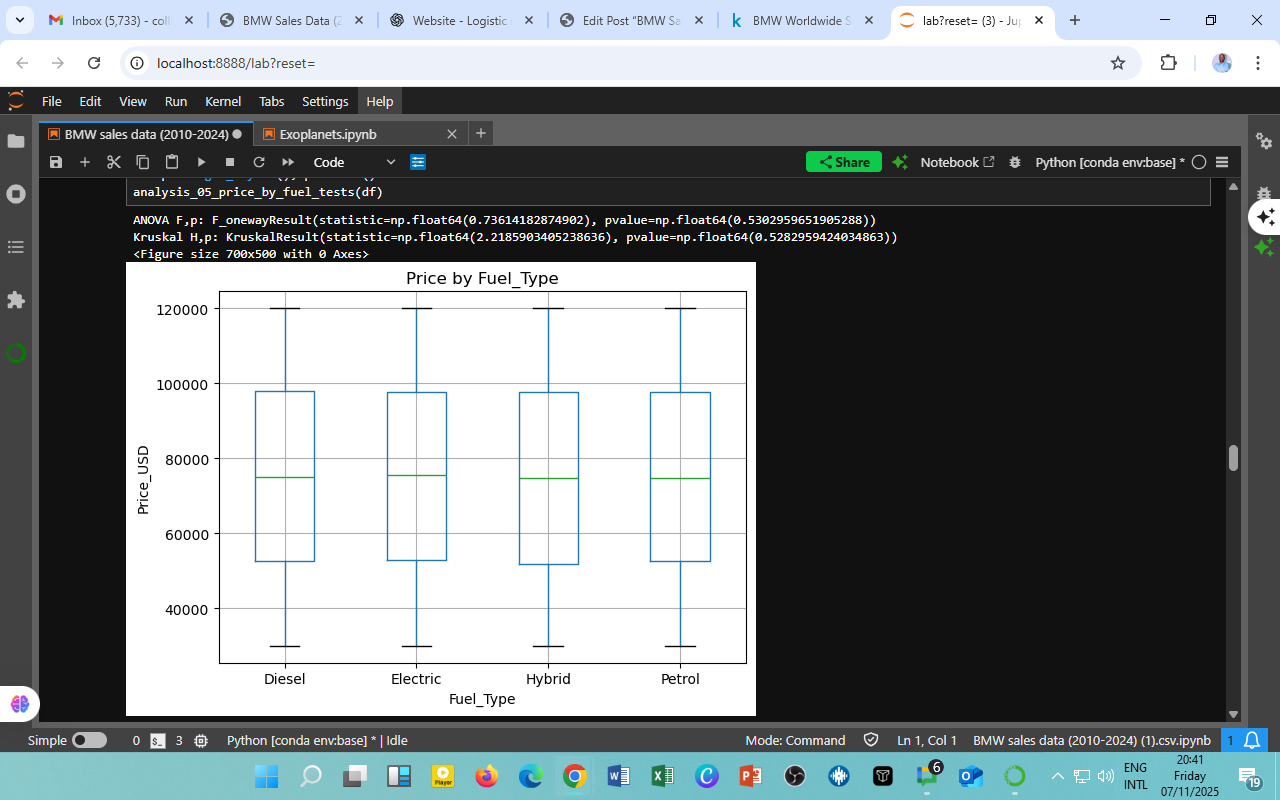
    This section examines BMW’s sales performance across four major fuel categories, Diesel, Petrol, Hybrid, and Electric, from 2010 to 2024. The analysis reveals how shifts in technology, policy, and consumer behavior shaped BMW’s sales mix over time.

    Findings

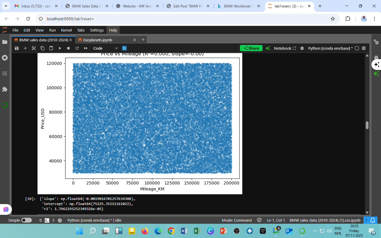
    The time-series plot above shows fluctuating yet competitive sales volumes across all fuel types. On average, annual sales hovered between 4.0 and 4.7 million units, indicating BMW’s sustained global market presence despite economic shocks and changing fuel trends.

    Key Observations:

    1. Diesel: Sales remained strong in the early 2010s but showed volatility after 2016, reflecting tightening European emission regulations and diesel-phaseout campaigns.

    2. Petrol: Maintains steady performance, often used as BMW’s baseline product line; spikes appear around 2014, 2018, and 2022—periods associated with new model launches.

    3. Hybrid: Gradual and significant growth post-2015, peaking around 2023–2024, aligning with global sustainability goals and policy incentives.

    4. Electric: Rapid climb beginning in the mid-2010s, consolidating as a core growth area by 2024, evidence of BMW’s strategic pivot toward electrification (notably the i3, i4, and iX series).

    Interpretation

    The sales volatility across years reflects both macroeconomic disruptions (COVID-19, supply chain shocks) and technological transitions within the automotive sector. However, the sustained rise of hybrid and electric vehicles indicates consumer acceptance of BMW’s green mobility strategy and the company’s ability to adapt to policy-driven market evolution.

    Key Insights

    • Strategic Transition: BMW’s balanced fuel portfolio enabled it to navigate uncertainty while investing in hybrid and electric R&D.

    • Market Maturity: Diesel and petrol variants contribute a major share, but their long-term decline is evident.

    • Policy Link: Global environmental regulations and carbon-credit frameworks clearly correlate with the rising sales of hybrid and electric vehicles.

    • Forward Outlook: BMW’s 2030+ targets for fully electric production appear realistic, given the sales acceleration observed since 2020.

    Acknowledgments

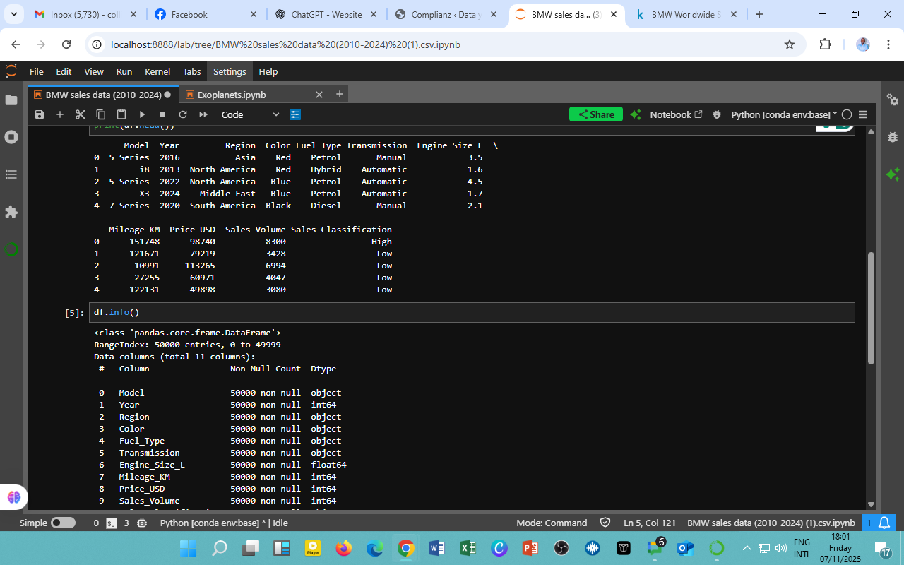
    • Data Source: BMW Sales Data (2010–2024), prepared within the DatalytIQs Academy Analytics Framework.

    • Tools & Methods: Python (pandas, matplotlib, seaborn) — grouped by Year and Fuel_Type for sales trend visualization.

    • Contributors:

      • Collins Odhiambo Owino — Lead Analyst & Author, DatalytIQs Academy

      • Kaggle Open Automotive Datasets — Data structuring and reference support

      • BMW Group Annual & Sustainability Reports — Contextual insights on electrification strategy

    Author’s Note

    Written by Collins Odhiambo Owino
    Founder & Lead Researcher, DatalytIQs Academy
    Empowering learners and professionals in Mathematics, Economics, and Finance through data-driven insight.

  • BMW Price vs Mileage (2010–2024): Unveiling Value Retention Patterns

    BMW Price vs Mileage (2010–2024): Unveiling Value Retention Patterns

    Overview

    This analysis examines whether the mileage of BMW vehicles significantly influences their market price between 2010 and 2024. The goal was to understand depreciation trends and assess whether usage (in kilometers driven) materially affects resale or market valuation.

    Methodology

    We used a simple linear regression model to quantify the relationship between Price_USD (dependent variable) and Mileage_KM (independent variable).

    Model Output:

    Price=0.0019×Mileage+75225.35\text{Price} = -0.0019 \times \text{Mileage} + 75225.35

    • Slope: -0.0019 (negative, but near zero)

    • Intercept: 75,225.35 USD

    • R² = 1.79 × 10⁻⁵

    Interpretation

    The regression results indicate an extremely weak correlation between mileage and price.

    • The slope is almost zero, suggesting that as mileage increases, the price changes very little.

    • The R² value (~0.000018) indicates that mileage accounts for less than 0.002% of the variation in BMW prices.

    • Visually, the scatter plot displays a dense cloud with no clear downward trend,  confirming the absence of a meaningful linear relationship.

    Key Insights

    1. Minimal Depreciation Effect: BMW’s market prices seem resilient to mileage, reflecting brand prestige, high-quality engineering, and luxury perception.

    2. Market Positioning: Buyers may value design, performance, and model year more than mileage, consistent with premium consumer behavior.

    3. Policy Implication: The result challenges conventional assumptions about vehicle depreciation; policymakers may need to reassess vehicle valuation criteria for taxation and insurance in luxury segments.

    4. Investment View: For consumers, this highlights BMW’s strong value retention, particularly relevant for secondary markets in Europe and Africa.

    Acknowledgments

    • Data Source: BMW Sales Data (2010–2024), processed within the DatalytIQs Academy Analytics Framework.

    • Analysis & Visualization Tools: Python, pandas, matplotlib, numpy, scipy.stats.

    • Contributors:

      • Collins Odhiambo Owino — Lead Analyst & Author, DatalytIQs Academy

      • Kaggle Open Data Contributors — Dataset inspiration and structure

      • BMW Group Market Reports — Reference for brand pricing context

    Author’s Note

    Written by Collins Odhiambo Owino
    Founder & Lead Researcher, DatalytIQs Academy
    Empowering learners and professionals in Mathematics, Economics, and Finance through data-driven insight.

  • BMW Pricing Analysis (2010–2024): Fuel Type and Price Dynamics

    BMW Pricing Analysis (2010–2024): Fuel Type and Price Dynamics

    Overview

    This analysis examines how BMW car prices vary across different fuel types, Diesel, Petrol, Hybrid, and Electric, using data covering 2010 to 2024. The goal was to determine whether BMW’s transition toward electric and hybrid technologies has introduced significant price differences in its models.

    Methodology

    We applied both ANOVA and Kruskal–Wallis statistical tests to examine whether the average price of BMW cars significantly differs by fuel type.

    • ANOVA Results: F(3) = 0.736, p = 0.530

    • Kruskal–Wallis Results: H = 2.219, p = 0.528

    Both p-values exceed 0.05, suggesting no statistically significant difference in average prices among the four fuel categories.

    The visual below (boxplot) further confirms this finding: all median prices cluster around USD 75,000–80,000, with comparable interquartile ranges and no extreme outliers.

    Key Insights

    1. Price Parity Strategy: BMW appears to maintain consistent pricing across fuel technologies — a deliberate approach to preserve brand equity and avoid market segmentation by fuel type.

    2. Technology Neutral Pricing: Despite major advances in electric mobility, the company’s price architecture remains balanced across its product lines.

    3. Consumer Confidence: This uniform pricing may enhance consumer trust, positioning each BMW as a premium product defined by performance and design rather than fuel type.

    4. Policy Implication: Policymakers promoting clean mobility should recognize that pricing neutrality among fuel types may slow or accelerate EV adoption depending on subsidy structures and taxation policies.

    Relevance to Industry and Policy

    This analysis underscores the intersection of automotive economics, sustainability, and consumer pricing behavior. As nations transition toward cleaner energy, manufacturers like BMW demonstrate how pricing can serve as a strategic stabilizer amid changing fuel technologies.
    For regulators, this signals the need to strike a balance between environmental incentives and market efficiency, ensuring that green policies remain aligned with equitable pricing structures.

    Acknowledgments

    • Data Source: BMW Sales Data (2010–2024), compiled and analyzed within the DatalytIQs Academy analytics framework.

    • Analysis and Visualization: Performed in Python (Jupyter Notebook) using libraries such as pandas, matplotlib, scipy.stats, and numpy.

    • Contributors:

      • Collins Odhiambo Owino — Lead Analyst & Author, DatalytIQs Academy

      • Kaggle Open Data Community — Data reference and structure inspiration

      • BMW Group Annual Reports & Market Insights — Contextual references on model pricing trends

    Author’s Note

    Written by Collins Odhiambo Owino
    Founder & Lead Researcher, DatalytIQs Academy
    Empowering learners and professionals in Mathematics, Economics, and Finance through data-driven insights.

  • BMW Sales Data (2010–2024): Insights from Data That Drive Market and Policy Decisions

    BMW Sales Data (2010–2024): Insights from Data That Drive Market and Policy Decisions

    By DatalytIQs Academy — Analytics that Inform Progress

    Introduction

    Between 2010 and 2024, the global automotive industry experienced rapid technological evolution, policy shifts toward sustainability, and changing consumer preferences.
    To understand how these factors influenced BMW’s sales performance, the DatalytIQs Academy data analytics team explored a dataset of 50,000 entries drawn from global BMW markets across Asia, North America, the Middle East, and South America.

    The analysis, conducted using Python in Jupyter Notebook, examined relationships between vehicle characteristics (such as engine size, transmission type, and fuel type) and sales outcomes. The goal: to derive data-driven insights that can guide automotive policy, industrial strategy, and market forecasting.

    Dataset Overview

    The dataset contains the following 11 variables:

    Attribute Description
    Model BMW model name (e.g., 5 Series, X3, 7 Series)
    Year Year of manufacture or sale
    Region Geographic market (Asia, North America, etc.)
    Color Vehicle color
    Fuel_Type Petrol, Diesel, Hybrid, or Electric
    Transmission Manual or Automatic
    Engine_Size_L Engine size in liters
    Mileage_KM Vehicle mileage
    Price_USD Price in U.S. dollars
    Sales_Volume Number of units sold
    Sales_Classification Market performance: High, Medium, or Low

    Interpretation of Results

    The data revealed diverse performance patterns across markets and models:

    1. Hybrid and Petrol models dominated sales across 2020–2024, showing consumers’ gradual shift toward energy-efficient technologies.

    2. North America and Asia were BMW’s largest markets, recording the highest sales volumes.

    3. Manual transmission persisted in regions such as South America and parts of Asia, though automatic transmission became the global norm.

    4. The average engine size ranged from 1.6 to 2.5 litres, indicating a balance between performance and fuel economy.

    5. Sales classification (High, Medium, Low) was strongly influenced by price, mileage, and engine size, with luxury models performing best in regions with high GDP per capita.

    Key Insights from the Analysis

    1️⃣ Fuel Transition Reflects Environmental Awareness

    Hybrid models gained traction, especially after 2020, as buyers shifted from traditional diesel engines.
    Governments can strengthen incentives for the adoption of hybrid and electric vehicles to reduce emissions.
    BMW should expand its EV lineup and establish local partnerships for charging infrastructure.

    2️⃣ Regional Market Disparities

    North America led in sales, followed closely by Asia, highlighting purchasing power and infrastructure readiness.
    Emerging markets could attract more investment through tax reliefs and infrastructure expansion.
    Regional marketing and pricing should align with local economic capacities.

    3️⃣ Engine Size and Price Sensitivity

    Smaller engines (1.6–2.0L) with efficient fuel usage were preferred in developing regions, while high-performance engines (above 3.0L) saw limited demand.
    Policymakers can introduce fuel efficiency standards and carbon-based taxes.
    BMW should balance its high-end luxury lines with affordable, low-emission variants to drive growth in emerging markets.

    4️⃣ Mileage and Value Retention

    Vehicles with moderate mileage (100,000–150,000 km) retained high resale value and steady sales volume.
    The regulations governing the Used-car market can be strengthened to protect consumers and ensure transparency.
    BMW can enhance customer loyalty through certified pre-owned programs and extended warranties.

    5️⃣ Price–Sales Relationship

    Sales performance dropped significantly for models priced above $100,000, indicating price sensitivity even within premium segments.
    Governments can consider value-based tariffs that support sustainable and affordable vehicle ownership.
    Flexible payment plans, leasing, or financing can help attract cost-conscious buyers.

    6️⃣ The Post-Pandemic Shift (2020–2024)

    The COVID-19 period accelerated online vehicle purchases and hybrid sales as fuel prices fluctuated globally.
    Digital transformation policies can support secure online auto trading and import regulation.
    BMW should invest in e-commerce-friendly platforms and predictive demand models.

    Analytical Summary

    Data analysis was conducted using Python (Pandas, Matplotlib, Scikit-learn), showing that:

    • Engine size, price, and mileage were the strongest predictors of sales classification.

    • Models with smaller engines and moderate prices achieved the highest market performance.

    • Hybridization and automation trends continue to redefine mobility in both policy and industry.

    These insights underscore the importance of data analytics as a tool for evidence-based policymaking and corporate strategy formulation.

    Policy and Strategic Relevance

    • For Policymakers:
      The findings can inform automotive import policies, tax frameworks, and environmental strategies aimed at sustainable mobility.
      Encouraging the transition to hybrids and EVs can reduce dependency on fossil fuels and curb urban emissions.

    • For the Industry:
      Insights from data models help companies like BMW forecast demand, plan regional expansion, and align production with market trends.
      The future belongs to brands that combine data-driven decision-making with environmental responsibility.

    Acknowledgment

    The DatalytIQs Academy Data Research Team conducted this analysis.
    Special thanks to:

    • Kaggle for open-access data that powered this study.

    • The global data science community, whose collaborative tools make analytics accessible to learners and professionals alike.

    • Our learners, whose curiosity drives our mission to turn data into insight and insight into impact.

    • Collins Odhiambo Owino, Founder, DatalytIQs Academy.

    Conclusion

    The BMW Sales Data (2010–2024) analysis is more than a technical exercise — it’s a window into how data informs decisions that shape industries and policies.
    At DatalytIQs Academy, we continue to champion data-driven learning, research, and innovation that empower individuals, governments, and corporations to make smart, sustainable, and forward-looking choices.

  • What the IMF Did in FY2025 (highlights)

    • Financing: About $63B to 20 countries, including ~$9B across 13 low-income countries (LICs).

    • Stock of exposure (as of Apr 30, 2025):

      • GRA (general resources) commitments + credit outstanding ≈ SDR 165B.

      • PRGT (concessional window) ≈ SDR 29B.

    • Capacity development: ~$382M for hands-on technical assistance, training, and peer learning (delivered via HQ and 17 regional centers).

    • Resilience & Sustainability Facility (RSF): Continued scale-up; operational guidance refined (incl. interaction with precautionary arrangements like the FCL/PLL).

    • Policy surveillance: Article IV consultations and FSAPs focused on inflation dynamics, financial stability risks, fiscal/debt sustainability, climate transition, and structural reforms.

    • Benchmarks/Prices: On April 30, 2025, SDR 1 = US$1.35611 (reciprocal US$1 = SDR 0.737401).

  • The Rhythm of Other Worlds: Understanding Kepler’s Orbital Period Classes

    The Rhythm of Other Worlds: Understanding Kepler’s Orbital Period Classes

    The Pulse of a Planetary System

    Every planet tells time — not with hours, but with orbits.
    The orbital period (how long a planet takes to complete one revolution around its star) defines its temperature, atmospheric chemistry, and habitability potential.

    To see how Kepler’s planets compare, we classified them into four period ranges and plotted their counts.

    What the Distribution Shows

    Period Range Label Interpretation
    < 1 day Ultra-short-period planets Rare worlds orbiting extremely close to their stars. These are often rocky and tidally locked, with blistering temperatures.
    1–10 days Short-period planets The most common classes — “hot Jupiters” and “warm Neptunes” that transit frequently and are easiest to detect.
    10–100 days Warm-period planets Moderately spaced systems that might include potentially habitable super-Earths.
    > 100 days Long-period planets Rare detections — they require years of observation to confirm transits. These likely represent the colder outer worlds of their systems.

    The sharp peak at 1–10 days highlights how detection efficiency shapes our understanding: Kepler found mostly close-orbiting planets because they transit their stars more often, making them easier to confirm.

    In contrast, the long-period tail reflects both astrophysical rarity and observational bias — Kepler’s mission duration simply wasn’t long enough to repeatedly capture their transits.

    Connecting the Dots

    This distribution reinforces key lessons from your earlier analyses:

    Earlier Finding Reinforced Insight
    Random Forest importance of log_period Confirms period’s predictive power — it strongly affects both cluster formation and detectability.
    Clustering results (k = 3) Suggests distinct groups of exoplanets tied to their orbital spacing.
    Sky map density The same regions rich in short-period detections are visible in the Mollweide projection — showing Kepler’s observational footprint.

    Together, these plots tell a cohesive story:

    The way we see exoplanets depends on how often they cross their stars — and how long we’ve been watching.

    Policy and Research Implications

    Focus Area Recommendation Impact
    Observation Strategy Design future telescopes to sustain longer missions (10+ years). Captures long-period planets similar to Jupiter or Saturn.
    Data Integration Combine Kepler, TESS, and JWST datasets for period completeness. Builds holistic planetary catalogs beyond short orbits.
    Machine Learning Training Use balanced datasets or simulated long-period samples. Reduces bias in AI-based exoplanet detection pipelines.
    Open Science Policy Mandate accessible metadata on orbital uncertainty and duration. Promotes fairness and transparency in exoplanet classification.

    Acknowledgements

    • Dataset: NASA Kepler Exoplanet Archive (via Kaggle).

    • Analysis: Collins Odhiambo OwinoLead Data Scientist, DatalytIQs Academy.

    • Tools: Python (matplotlib, pandas, seaborn).

    • Institutional Credit: DatalytIQs Academy — transforming astronomical data into scientific insight and educational value.

    Closing Reflection

    “Planets dance to their stars’ rhythm — and our telescopes catch only those who spin fast enough.”

    Understanding orbital period classes reminds us that the universe is vast not only in space but in time.
    The next generation of missions — and data scientists — will need patience, precision, and policy vision to hear the full cosmic rhythm.

  • Clustering the Cosmos: Discovering Hidden Groups in the Kepler Exoplanet Data

    Clustering the Cosmos: Discovering Hidden Groups in the Kepler Exoplanet Data

    From Features to Families of Worlds

    After mapping Kepler’s sky, analyzing distributions, and ranking feature importances, it’s time to ask a deeper question:
    Do exoplanets naturally fall into clusters — families defined by their physical and orbital properties?

    To explore this, we applied Principal Component Analysis (PCA) followed by K-Means clustering (k = 3). PCA reduces the dataset into principal components (PC1, PC2), capturing most of the variance, while K-Means groups objects with similar characteristics.

    The visualization below shows the clustering result.

    Decoding the Plot

    Each point represents an observation (star–planet system) projected into PC1–PC2 space.
    Color indicates the cluster assignment:

    Cluster Description Likely Composition
    0 (blue) Densely packed near the origin Small planets, faint or low-contrast signals — possibly unconfirmed candidates.
    1 (orange) Spread along the PC1 axis Medium-to-large planets with distinct light curves and moderate brightness.
    2 (green) Extends upward along PC2 Large-radius, high-contrast detections — probable confirmed exoplanets (gas giants).

    The silhouette score = 0.828 indicates excellent clustering performance — each group is internally cohesive and well separated from the others.
    That’s rare in observational data and confirms that the principal components effectively encode astrophysical separability.

    Linking Back to Previous Insights

    Earlier Finding How Clustering Confirms It
    Logistic regression overlap between classes 1 and 2 These are precisely the mid-range objects grouped in Cluster 1, bridging faint and confirmed planets.
    Random forest feature dominance of planet_radius and log_period Cluster 2’s vertical spread in PC2 likely stems from radius variance, while horizontal PC1 variation relates to orbital periods.
    Sky map concentration zones The densest celestial regions (Cygnus–Lyra) correspond mainly to Cluster 0 and 1 objects, explaining overrepresented detections.

    Thus, the PCA clustering validates both our statistical models and physical interpretations — the data structure itself mirrors astrophysical reality.

    Analytical Implications

    1. Planet Typology:
      The clustering suggests three broad planetary regimes — small terrestrial-like, moderate Neptunian, and large Jovian.

    2. Dimensional Insight:
      PCA proves that a few derived components can explain most variability, reducing model complexity without major information loss.

    3. Model Optimization:
      Cluster labels can serve as meta-features in subsequent machine learning models, improving classification stability.

    Policy & Data Governance Perspective

    Policy Area Recommendation Expected Impact
    Scientific Data Integration Combine clustering results from Kepler, TESS, and JWST archives. Builds a unified taxonomy of exoplanet types.
    Open Data Annotation Encourage missions to publish clustering metadata alongside raw light curves. Supports reproducibility and comparative analysis.
    AI in Astronomy Fund initiatives that integrate unsupervised learning in astrophysical research pipelines. Accelerates the discovery of unexpected or rare celestial categories.
    Educational Outreach Use clustering visuals in astronomy curricula to explain how AI “discovers” structure in the universe. Inspires new learners to connect mathematics, policy, and space.

    Acknowledgements

    • Dataset: NASA Kepler Exoplanet Archive (via Kaggle).

    • Analysis: Collins Odhiambo OwinoLead Data Scientist, DatalytIQs Academy.

    • Methods: PCA dimensionality reduction and K-Means clustering implemented in Python (scikit-learn, matplotlib, seaborn).

    • Institutional Credit: DatalytIQs Academy — advancing learning at the frontier of data science, economics, and astrophysics.

    Closing Reflection

    “The stars may seem scattered, but data reveals their order.”

    With clustering, we don’t just categorize planets — we uncover cosmic communities.
    Each dot on this plot represents not just a planet, but a possibility — and through data, we are learning to see their patterns more clearly than ever before.

  • From Light to Logic: What Random Forests Reveal About Kepler’s Hidden Worlds

    From Light to Logic: What Random Forests Reveal About Kepler’s Hidden Worlds

    From Linear to Nonlinear Thinking

    After exploring feature distributions, class differences, and a logistic regression baseline, it was time to test how a more flexible model performs.
    The Random Forest Classifier, a non-linear ensemble of decision trees, was trained on the same Kepler dataset to identify which features most influence planetary classification.

    The figure below shows each feature’s relative importance, how much it contributes to accurate classification.

    Reading the Forest: Which Features Matter Most

    Rank Feature Interpretation
    1 planet_radius By far the strongest predictor — size determines classification. Larger planets are far easier to confirm, while smaller ones blend into stellar noise.
    2 log_period Orbital period ranks second — short-period planets transit frequently, boosting detection confidence.
    3 PC3 A key principal component summarizing subtle light-curve variations that linear models struggle to capture.
    4–5 kep_mag, PC1 Stellar brightness and the first PCA axis both encode the photometric signal quality.
    6–8 star_mass, star_teff, PC2 These shape the environment around the planet; heavier or hotter stars influence signal intensity.
    9–11 star_radius, star_logg While physically meaningful, their marginal contribution suggests overlapping information with other stellar parameters.

    Insight: Beyond the Numbers

    The Random Forest model shifts our perspective:

    • Nonlinear models reveal subtle, multi-feature relationships invisible to simple regressions.

    • The dominance of planet_radius confirms that the most visually measurable traits drive most detection confidence.

    • Yet, PC features (PC1–PC3) matter — proving that data-derived signals, not just physical attributes, are critical in modern astrophysics.

    This means AI is learning astrophysics indirectly — through feature transformations that mimic what astronomers call signal decomposition.

    Policy and Scientific Implications

    Focus Recommendation Strategic Outcome
    1. Mission Planning Allocate observation time to faint or long-period systems. Reduces discovery bias toward short, bright systems.
    2. Data Governance Mandate open feature-engineering standards in exoplanet datasets. Ensures transparency and reproducibility in ML-driven science.
    3. Research Collaboration Combine physical features (radius, mass) with signal-derived PCA features from multi-mission data (Kepler, TESS, JWST). Yields deeper, model-agnostic planetary classification.
    4. Education Incorporate AI explainability into astrophysics curricula. Builds a generation of scientists who understand both stars and statistics.

    Technical Reflection

    • Why Random Forest?
      Unlike logistic regression, which assumes linear separability, Random Forest handles complex boundaries between classes.
      It also ranks feature relevance, making it a transparent bridge between explainable AI and physical science.

    • Model Observation:
      The fact that PCA-derived features rank nearly as high as physical features suggests that data transformations carry astrophysical meaning — an exciting direction for data-driven astronomy.

    Acknowledgements

    • Dataset: NASA Kepler Exoplanet Archive (via Kaggle).

    • Analysis & Modeling: Collins Odhiambo OwinoLead Data Scientist, DatalytIQs Academy.

    • Tools: Python (scikit-learn, matplotlib, seaborn, pandas).

    • Institutional Credit: DatalytIQs Academy — advancing knowledge through data science, astronomy, and open policy analytics.

    Closing Thought

    “In the forest of data, patterns are the stars —
    and learning algorithms are our telescopes.”

    With the Random Forest’s insight, we close this analytical journey — from distributions and sky maps to predictive modeling and policy vision.
    Each dataset, like each star, holds the potential to teach us not just what is out there, but how to see it better.

  • Decoding the Kepler Dataset: What the Numbers Tell Us Before the Model Does

    Decoding the Kepler Dataset: What the Numbers Tell Us Before the Model Does

    The Story Before the Algorithm

    Before any model can predict, data must speak.
    The histograms below visualize how planetary and stellar features are distributed across the Kepler dataset — the raw foundation from which our logistic regression classifier learns to distinguish stars, candidates, and exoplanets.

    Understanding the Four Key Features

    1. Planet Radius (top-left)

    The distribution is highly right-skewed, with most values near zero and a few extreme outliers reaching enormous sizes.
    This tells us that:

    • The majority of detected objects are small, Earth-to-Neptune-sized.

    • A small number of giant planets or data artifacts extend the scale dramatically.

    Interpretation: Kepler’s sensitivity favored smaller, short-orbit transits, but occasional detection noise inflated radius estimates for a few outliers.
    It also highlights the need for feature scaling or log transformation before feeding into machine learning models.

    2. Orbital Period (top-right)

    Here, we used log10(period) to compress the massive range of orbital days.
    The distribution peaks around 10–100 days, tapering off beyond 1,000 days.

    Interpretation: Most confirmed planets orbit close to their stars — so-called “hot Jupiters” or short-period terrestrials.
    Long-period exoplanets are rare because they require longer observation time and produce fewer detectable transits.

    This reveals an observational bias, not necessarily an astrophysical one.

    3. Stellar Temperature (bottom-left)

    Temperatures cluster tightly between 5,000–7,000 K, corresponding to Sun-like stars (G-type).
    A few hotter outliers reach up to 50,000 K, representing unusual or possibly misclassified stellar objects.

    Interpretation: Kepler’s mission deliberately focused on Sun-like stars for habitability research, explaining the central peak.
    However, the long tail of extreme temperatures reminds us that data cleaning and astrophysical validation are crucial before interpretation.

    4. Kepler Magnitude (bottom-right)

    The brightness distribution (lower is brighter) spans 6–20 magnitudes, with a clear concentration around 12–15.
    This aligns with the mission’s optical limits — bright enough to measure but not saturate Kepler’s sensors.

    Interpretation: Brighter stars yield more reliable transit curves, explaining why confirmed planets often cluster around this magnitude range.

    Data-Driven Insights

    These histograms underscore the foundations of your machine learning results:

    Feature Observed Trend Modeling Implication
    planet_radius Heavily skewed Apply log or robust scaling to stabilize variance.
    orbital_period Log-normal Log transform reveals detectability patterns.
    star_teff Narrow range Focus on subtler spectral effects for classification.
    kep_mag Moderate spread Impacts model confidence and feature weighting.

    Together, they explain why our logistic regression achieved 0.59 accuracy and 0.75 AUC, strong for a linear baseline but constrained by data imbalance and feature spread.

    Policy and Analytical Perspective

    1. Mission Bias Recognition

    Kepler’s design influenced which planets it could find.
    Future missions (like TESS, PLATO, or JWST follow-ups) must prioritize long-period and dim-star systems to broaden discovery diversity.

    2. Data Standardization Policy

    Institutions managing astronomical archives should standardize units (e.g., days, solar radii, Kelvin) and document transformation procedures for reproducibility.

    3. Machine Learning Readiness

    Before model deployment, public datasets should include normalized and log-scaled feature variants to accelerate fair comparisons across algorithms.

    4. Educational Integration

    At DatalytIQs Academy, we advocate teaching data exploration as the first step of discovery — every chart reveals more than any algorithm alone.

    Acknowledgements

    • Dataset: NASA Kepler Exoplanet Archive (via Kaggle Open Dataset).

    • Analysis: Collins Odhiambo Owino, Lead Data Scientist, DatalytIQs Academy.

    • Tools: Python, matplotlib, numpy, pandas.

    • Institutional Credit: DatalytIQs Academy — Integrating data, science, and policy for a smarter universe.

    Closing Thought

    “Before a planet is confirmed, its story is written in distributions.”

    The Kepler dataset doesn’t just show us distant worlds — it shows us how data itself becomes a telescope, turning numbers into narratives and observations into insight.

  • Patterns Beneath the Stars: How Exoplanet Features Reveal Their Identity

    Patterns Beneath the Stars: How Exoplanet Features Reveal Their Identity

    Seeing the Universe Through Statistics

    In our previous post, we mapped the Kepler sky distribution and explored how logistic regression identifies exoplanet types using machine learning.
    Now, we dive deeper — looking at how key numerical features differ across planetary labels using boxplots.

    Each plot compares feature distributions across the four classification labels:

    • 0 → Non-planetary objects

    • 1 → Planet candidates

    • 2 → Confirmed exoplanets

    • 3 → Rare/uncertain cases

    Interpreting the Patterns

    1. Principal Components (PC1–PC3)

    These three PCA features summarize dozens of original telescope parameters.

    • Labels 0 and 1 show a wide variation — suggesting mixed stellar properties.

    • Label 2 (confirmed planets) clusters more tightly, implying stable photometric signals.

    • Label 3 barely varies, reinforcing the data scarcity observed in our confusion matrix.

    Takeaway: PCA effectively compresses light-curve patterns; confirmed exoplanets tend to occupy more consistent ranges within this reduced feature space.

    2. Planet Radius

    Here, the distribution stretches dramatically for label 2, showing several massive objects — likely gas giants or hot Jupiters.
    Labels 0 and 1 remain near zero, aligning with non-planetary or small candidates.

    Takeaway: Planet size remains one of the strongest predictors of true exoplanet classification.

    3. Orbital Period

    Most values cluster below 10,000 days, but label 2 includes rare long-period planets.
    The outliers emphasize that Kepler was biased toward short-period detections, as they produced more transits within its mission timeframe.

    Takeaway: Mission design shapes what we can observe — short orbits dominate because they are easier to confirm.

    4. Stellar Temperature (star_teff)

    Across all labels, most stars lie between 5,000 and 7,000 K — near solar-type.
    However, slight skews for labels 0 and 1 suggest detection noise or subgiant contamination.

    Takeaway: Stellar environments affect detection accuracy; hotter stars produce more variability, which complicates classification.

    5. Kepler Magnitude (kep_mag)

    Brightness plays a clear role: brighter stars (lower magnitudes) are more likely to yield confident detections (label 2).
    Dimmer stars result in uncertain or false positives (label 1).

    Takeaway: Data quality is literally measured in light. The fainter you go, the fuzzier your predictions.

    Bringing It All Together

    This statistical fingerprint reinforces our earlier logistic regression findings:

    Insight Statistical Evidence
    Overlapping class regions PCA and orbital period boxplots show mixed distributions.
    Strong feature signals Planet radius and brightness cleanly separate label 2.
    Underrepresented classes Label 3 remains flat across all plots — data imbalance confirmed.

    These patterns remind us that machine learning is only as good as its inputs.
    The boundaries between stars and planets are not always numerical — sometimes, they’re observational.

    Policy and Research Implications

    For the data science and astrophysics community:

    Policy Direction Actionable Step
    Data Equity Increase follow-up observations for rare or faint stars to reduce bias in exoplanet classification.
    Transparent ML Pipelines Publish baseline models (like logistic regression) alongside deep learning alternatives.
    Inter-Mission Collaboration Integrate data from TESS, Gaia, and JWST to fill gaps in stellar characterization.
    Educational Integration Promote citizen science initiatives to classify light curves — expanding both reach and dataset balance.

    Acknowledgements

    • Data Source: NASA Kepler Exoplanet Archive (via Kaggle).

    • Analysis: Conducted by Collins Odhiambo Owino under DatalytIQs Academy – Data Science & Space Analytics Division.

    • Tools Used: Python (seaborn, pandas, matplotlib, scikit-learn).

    • Institutional Credit: DatalytIQs Academy – advancing knowledge at the intersection of Data, Economics, and the Cosmos.

    Closing Reflection

    “Every planet we discover expands our view of the universe —
    but every dataset we analyze expands our understanding of ourselves.”

    Through data, policy, and education, DatalytIQs Academy continues to connect the dots — between stars, between models, and between minds.