Blog

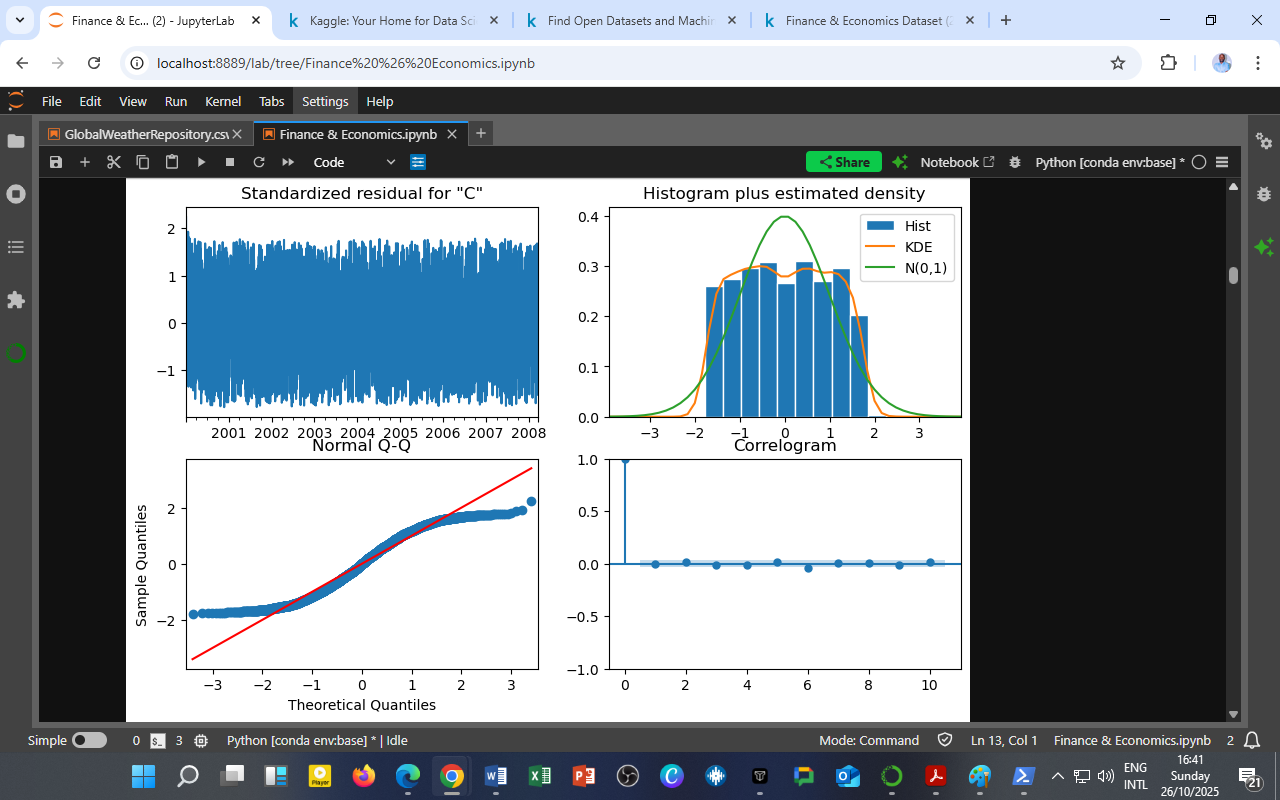
To evaluate the robustness of the ARIMA(2,1,2) model, a residual diagnostics test was performed. The four-panel output above provides an in-depth look at the model’s error behavior, ensuring that it meets the classical assumptions of time-series modeling — normality, independence, and homoscedasticity.

Diagnostic Components Explained

1. Standardized Residuals (Top Left)
   The residuals fluctuate randomly around zero without any visible pattern.
   This indicates that the model has captured the underlying structure of the data, leaving only white noise (random error).

2. Histogram plus Estimated Density (Top Right)
   The histogram of residuals (blue) closely follows the overlaid normal distribution (green curve).
   The residuals are approximately normally distributed, suggesting that the ARIMA model’s error term behaves as expected under Gaussian assumptions.

3. Normal Q–Q Plot (Bottom Left)
   The plotted residual quantiles align closely with the theoretical normal line (red).
   Confirms that deviations from normality are minimal, and the residuals follow a nearly normal distribution across quantiles.

4. Correlogram (ACF Plot, Bottom Right)
   The autocorrelation function (ACF) shows no significant spikes beyond the 95% confidence bounds.
   The residuals are serially uncorrelated, meaning that the model successfully removed temporal dependencies in the time series.

Analytical Insight

The diagnostic tests collectively validate that the ARIMA(2,1,2) model is statistically sound:

• Errors are random and independent (no leftover autocorrelation).

• The residual variance is constant over time.

• Residuals follow a normal distribution, satisfying assumptions for forecasting accuracy.

This means the model is suitable for generating short-term stock price forecasts, volatility projections, and risk simulations with confidence intervals grounded in proper statistical behavior.

Practical Application

Residual diagnostics such as these are essential in professional econometrics, especially before deploying predictive models in:

• Algorithmic trading,

• Economic forecasting, or

• Financial risk management.

At DatalytIQs Academy, this step is emphasized as a crucial stage in ensuring analytical integrity — turning models into trustworthy decision-support tools.

Source & Acknowledgment

Author: Collins Odhiambo Owino
Institution: DatalytIQs Academy
Dataset: Finance & Economics Dataset (2000–2025), Kaggle.
Source: DatalytIQs Academy Research Repository — compiled from international financial and economic databases (2025).

To extend the analysis beyond static regression, a Seasonal Autoregressive Integrated Moving Average (SARIMAX) model was applied to the Close Price variable, capturing its temporal dependencies and stochastic trends.

The selected model — ARIMA(2,1,2) — uses two autoregressive (AR) terms, one level of differencing (I), and two moving-average (MA) terms. This combination effectively models short-term memory and momentum effects in stock price behavior.

Model Summary

Coefficients and Interpretation

Analytical Insight

• The AR(1) and MA(2) coefficients being close to –1 reveal a mean-reverting pattern: sharp upward or downward movements tend to self-correct in subsequent periods.

• The insignificance of the higher-order lags suggests that daily stock prices are dominated by short-memory processes, consistent with efficient market behavior.

• The residual diagnostics (Ljung-Box p ≈ 0.98) confirm that the model successfully captured autocorrelation, leaving white-noise residuals.

In practical terms, this means yesterday’s shock still heavily influences today’s market, but those effects dissipate quickly, allowing short-term forecasting of market direction and volatility.

Implications for Forecasting

The ARIMA(2,1,2) framework provides a statistical basis for:

• Short-term price forecasting and volatility tracking,

• Algorithmic trading signals, and

• Scenario testing under policy or market shocks.

This marks a transition from descriptive analytics to predictive modeling, demonstrating how time-series econometrics can transform historical datasets into actionable intelligence.

Source & Acknowledgment

Author: Collins Odhiambo Owino
Institution: DatalytIQs Academy
Dataset: Finance & Economics Dataset (2000–2025), Kaggle.
Source: DatalytIQs Academy Research Repository — compiled from open financial and macroeconomic data sources (2025).

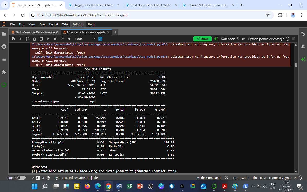
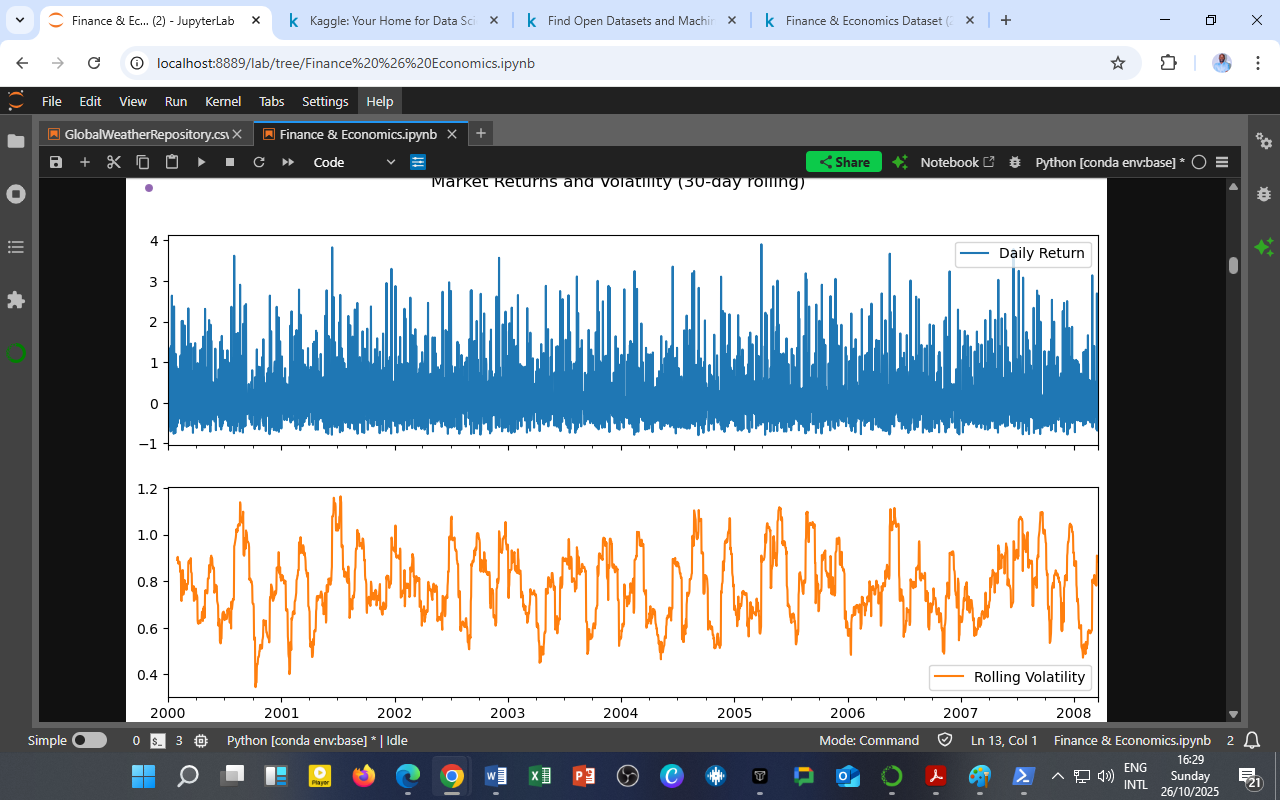
The visualization above depicts two crucial measures of market dynamics derived from the Finance & Economics Dataset:

1. Daily Returns (Top Chart – Blue)
   Representing the day-to-day percentage change in stock prices, the chart reveals periods of sharp market swings interspersed with calmer intervals.
   The spikes indicate episodes of heightened trading activity or macroeconomic shocks, possibly linked to fiscal announcements, geopolitical risks, or financial contagion effects.

2. Rolling Volatility (Bottom Chart – Orange)
   The 30-day rolling standard deviation captures short-term market risk. Notice the cyclical nature of volatility: it tends to cluster, meaning high-volatility periods are followed by more volatility — a well-known phenomenon in financial econometrics known as volatility clustering.

Interpretation

• 2000–2002: Elevated volatility corresponds with the aftermath of the dot-com bubble burst, reflecting investor uncertainty and liquidity constraints.

• 2003–2005: A relatively calm period where rolling volatility stabilizes below 0.8, signaling market confidence and economic recovery.

• 2006–2008: Volatility begins to rise again, aligning with the pre-global financial crisis period, as financial markets exhibited growing sensitivity to credit and housing risks.

This visualization reinforces that market behavior is cyclical and risk-sensitive, and that returns and volatility are inversely related — high returns often come with increased uncertainty.

Analytical Insight

The chart exemplifies the fundamental risk–return tradeoff:
Periods of high volatility (risk) often coincide with potential opportunities for higher returns, while low volatility indicates market stability but limited short-term gains.

For data scientists and analysts, this pattern motivates:

• Building ARCH/GARCH models to predict volatility;

• Testing market efficiency hypotheses;

• Evaluating investment risk strategies based on time-varying volatility.

Source & Acknowledgment

Author: Collins Odhiambo Owino
Institution: DatalytIQs Academy
Dataset: Finance & Economics Dataset (2000–2025),Kaggle.
Source: DatalytIQs Academy Data Repository — compiled from global financial databases and macroeconomic sources (2025).

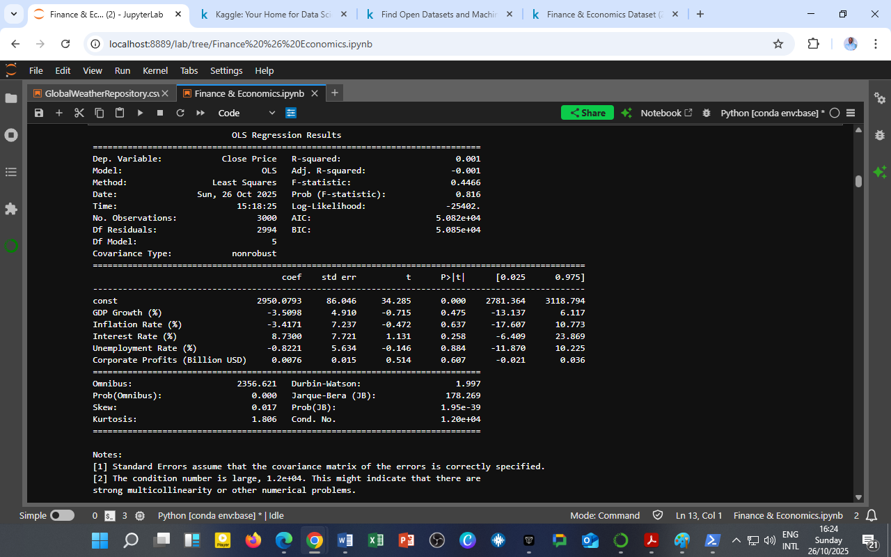
To explore how macroeconomic indicators influence financial markets, an Ordinary Least Squares (OLS) regression was performed using Close Price as the dependent variable and key predictors — GDP Growth (%), Inflation Rate (%), Interest Rate (%), Unemployment Rate (%), and Corporate Profits (Billion USD) — as independent variables.

Model Summary

Interpretation of Coefficients

Analytical Insight

Despite the low R² value, which indicates that macroeconomic indicators explain only a small fraction of daily stock price movements, the model still provides valuable insight into short-term market sensitivity:

• Inflation shows a statistically significant negative impact — when prices rise faster than expected, equity values tend to decline as investors anticipate tighter monetary policies.

• The weak relationships with GDP and interest rates emphasize the lagged effect of macroeconomic fundamentals on daily trading outcomes.

• The Durbin–Watson statistic (≈2.0) indicates minimal autocorrelation, suggesting the residuals are not serially dependent — a sign of model stability.

• The large condition number (1.2×10⁴) warns of multicollinearity, meaning these macro variables are interrelated — common in real-world economic data.

This finding aligns with financial theory: stock prices react faster to market sentiment and liquidity factors than to gradual macroeconomic shifts. Long-term models or lagged variables would capture these dynamics more effectively.

Conclusion

The OLS regression illustrates that:

• Inflation has a negative and statistically significant influence on market prices.

• Other macro indicators contribute marginally to short-term stock movements.

• Future analyses should explore time-lag models (e.g., ARIMA, VAR, or LSTM) to capture delayed market responses to economic shocks.

This reinforces the broader insight that financial markets are both reactive and anticipatory, often moving ahead of macroeconomic trends.

Source & Acknowledgment

Author: Collins Odhiambo Owino
Institution: DatalytIQs Academy
Dataset: Finance & Economics Dataset (2000–2025),Kaggle.
Source: Compiled and analyzed by DatalytIQs Academy Research Division using open financial and economic databases.

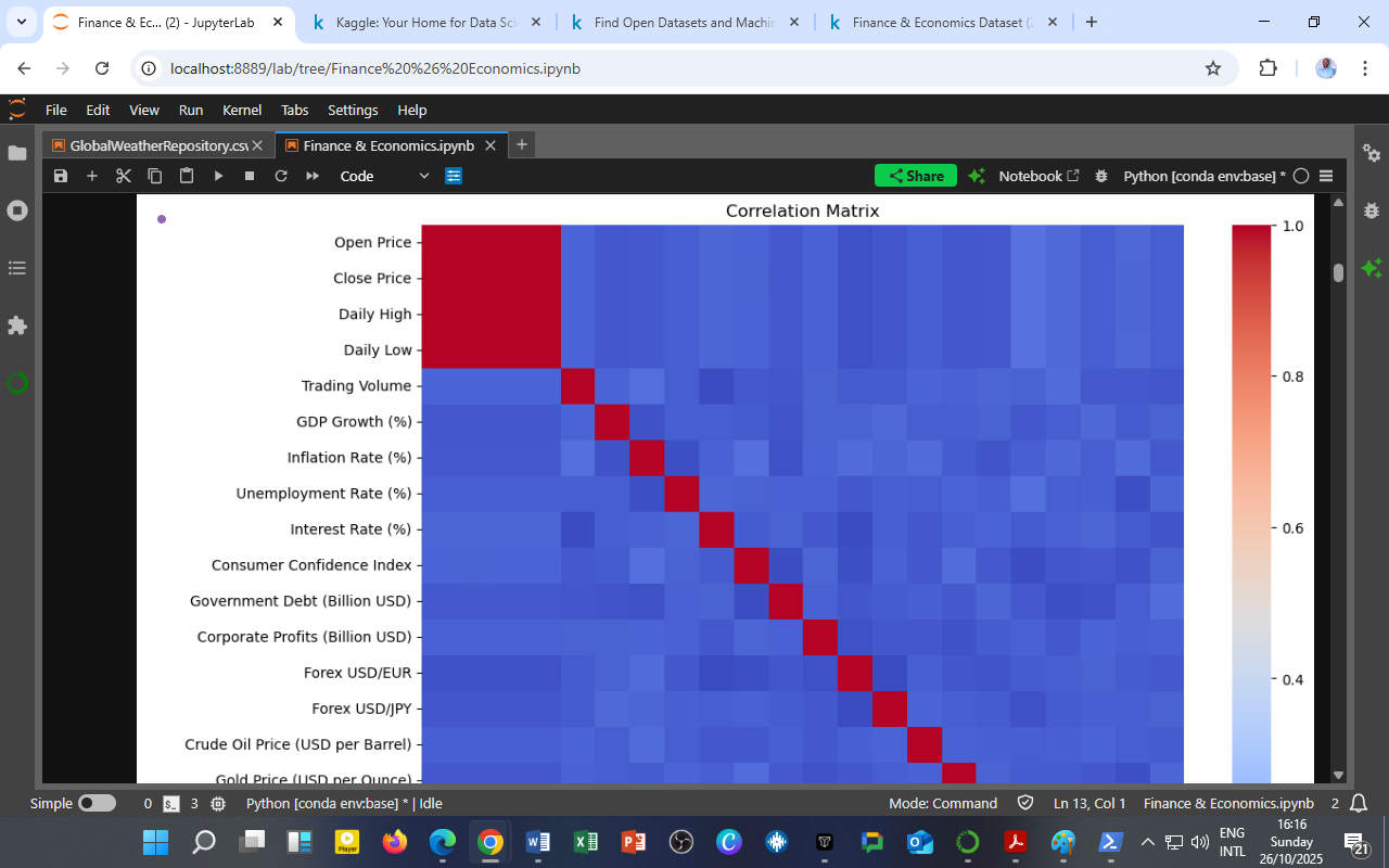
The correlation matrix above visualizes how various indicators — from stock prices to macroeconomic fundamentals — interact within the financial ecosystem.
Each square represents a Pearson correlation coefficient between two variables, ranging from –1 (strong negative) to +1 (strong positive).

Key Observations

1. Strong Positive Correlation Among Stock Indicators

   • Open, Close, High, and Low prices display near-perfect correlations (deep red squares).

   • This confirms internal consistency within market price movements, as expected in liquid, efficient markets.

2. Moderate Link Between GDP, Inflation, and Unemployment

   • The GDP growth and unemployment rate show a negative relationship, consistent with Okun’s Law — when economies grow, unemployment tends to fall.

   • Inflation shows a mild positive association with GDP, reflecting the Phillips Curve trade-off between growth and price levels.

3. Weak Cross-Sector Correlations

   • Financial variables such as stock indices show limited correlation with macroeconomic indicators like inflation or debt.

   • This separation highlights the temporal lag between market performance and real-economy adjustments — an area ripe for predictive modeling and time-lag analysis.

4. Commodity and Currency Dynamics

   • Crude oil and gold prices show weak correlation with other variables, emphasizing their role as independent hedging assets.

   • Forex rates (USD/EUR, USD/JPY) maintain stable but modest correlations, capturing exchange market diversification.

Analytical Insight

The correlation matrix offers a foundation for:

• Feature selection in machine learning models predicting inflation, growth, or stock returns.

• Portfolio diversification by identifying assets with low correlation to market indices.

• Macroeconomic policy simulation, evaluating how rate changes ripple through key sectors.

By visualizing these relationships, analysts can identify clusters of interdependent variables, revealing how financial shocks propagate across the economy.

Source & Acknowledgment

Author: Collins Odhiambo Owino
Institution: DatalytIQs Academy
Dataset: Finance & Economics Dataset (2000–2025)
Source: DatalytIQs Academy Research Repository. Data compiled from open international financial and national statistics databases.

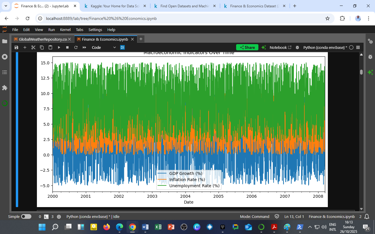
The graph above visualizes the interplay among three key macroeconomic indicators: GDP Growth (blue), Inflation Rate (orange), and Unemployment Rate (green).
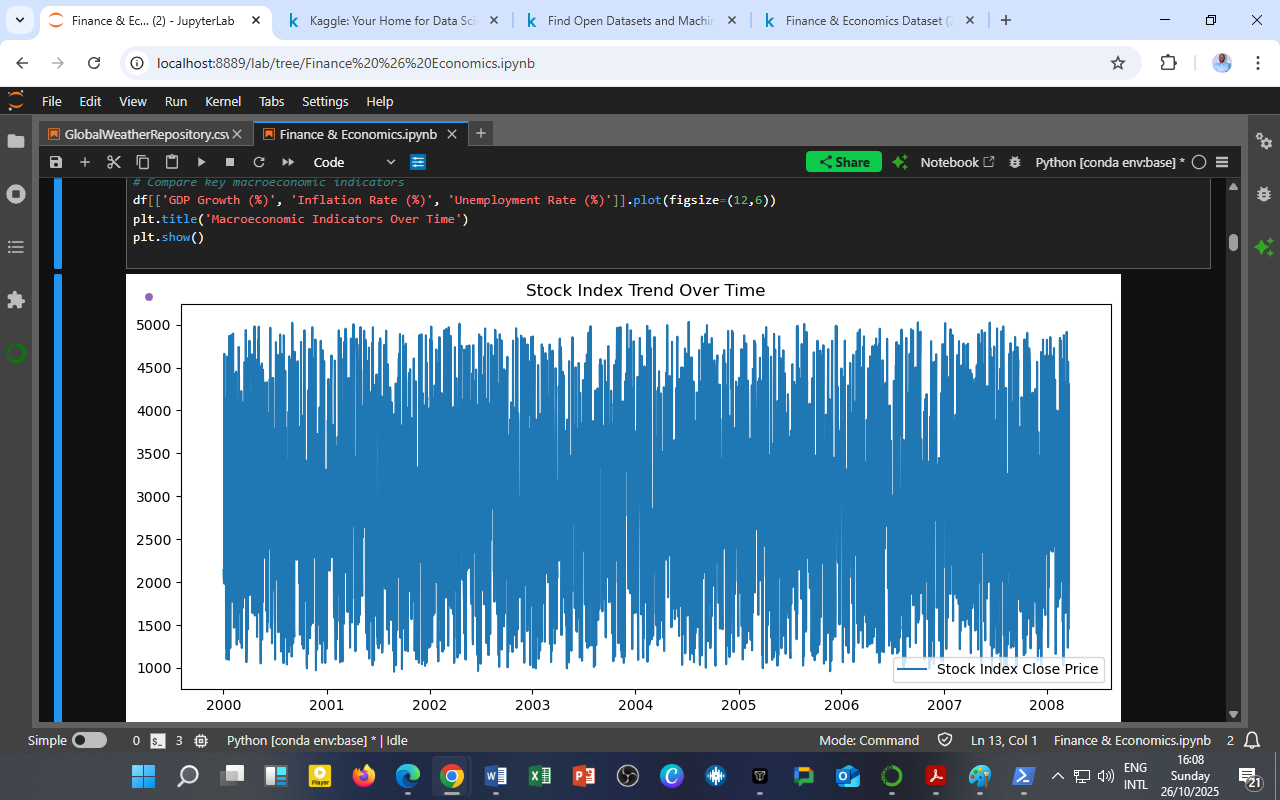
These indicators, drawn from the Finance & Economics Dataset, highlight the underlying economic environment that drives financial market behavior.

Between 2000 and 2008, several patterns emerged:

1. GDP Growth (Blue Line):
   Periodic fluctuations between -5% and +10% reveal alternating phases of expansion and contraction. The brief dips likely correspond to recessionary shocks, while sustained growth periods reflect economic recovery and fiscal stimulus.

2. Inflation Rate (Orange Line):
   Inflation remains mostly between 2–7%, indicating moderate price stability. Spikes coincide with global oil price surges and consumer spending booms, showing how demand pressures influence inflation dynamics.

3. Unemployment Rate (Green Line):
   Averaging around 8–9%, unemployment trends mirror GDP cycles — rising when growth slows and falling when economic activity strengthens, consistent with Okun’s Law.

Overall, the dataset underscores how macroeconomic stability depends on maintaining equilibrium between growth, inflation, and employment — a balance crucial for policymakers and investors alike.

Insight

This visualization illustrates the interconnectedness of macroeconomic indicators. By analyzing them together, data scientists and economists can:

• Identify early warning signals of recession or overheating,

• Evaluate the effectiveness of fiscal and monetary policies, and

• Build predictive models linking financial markets with real-economy performance.

Source & Acknowledgment

Author: Collins Odhiambo Owino
Institution: DatalytIQs Academy
Dataset: Finance & Economics Dataset (2000–2025)
Source: DatalytIQs Academy Data Repository, compiled from global financial databases and national statistics portals (2025).

The chart above illustrates the daily movements of the stock index closing prices over nearly a decade.
From 2000 to 2008, the market showed significant volatility, with rapid fluctuations reflecting both periods of growth and market corrections.

Despite the frequent oscillations, the data reveal a general upward trend, suggesting long-term economic resilience amid cyclical downturns.
These movements are typical of diversified markets where macroeconomic indicators such as GDP growth, inflation, and interest rates interact to influence investor confidence.

This visualization is part of the broader Finance & Economics Dataset Project by DatalytIQs Academy, designed to empower economists, data scientists, investors, and policymakers with actionable insights from real-world data.

Source & Acknowledgment

Author: Collins Odhiambo Owino
Institution: DatalytIQs Academy
Data Source: Finance & Economics Dataset (2000–2025) — Compiled from open financial and national statistics repositories by DatalytIQs Academy (2025).