Blog

  • Lag Correlation Between Consumer Confidence and Spending

    Lag Correlation Between Consumer Confidence and Spending

    Quantifying Behavioral Response Times in the Economy (2000–2008)

    By Collins Odhiambo Owino
    Founder & Lead Analyst — DatalytIQs Academy
    Source: Finance & Economics Dataset (2000–2025), DatalytIQs Academy Research Repository

    Introduction

    In behavioral economics, confidence drives spending — but the response is rarely instant.
    Consumers tend to adjust their expenditure after confirming improvements in job security, wages, or prices.
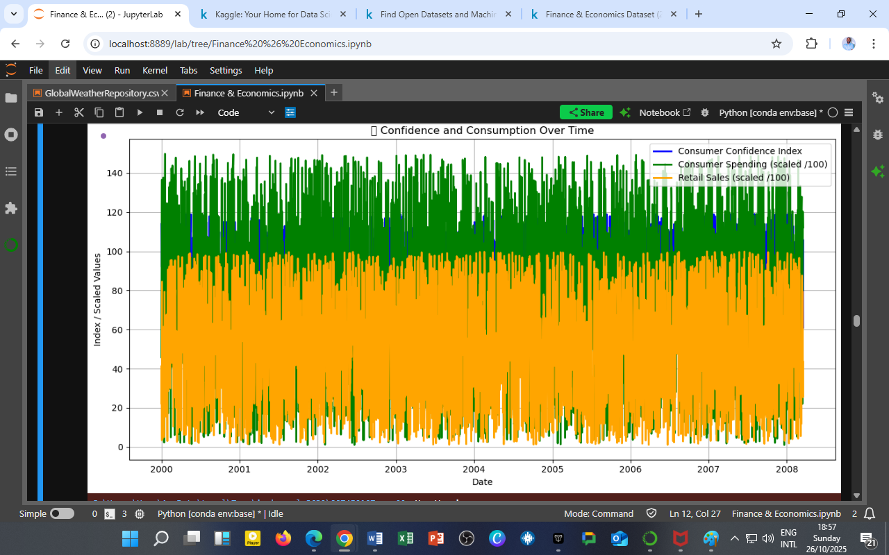
    To uncover this delayed behavioral pattern, we use a lag correlation analysis between the Consumer Confidence Index and Consumer Spending (Billion USD).

    Visualization: Lag Correlation Plot

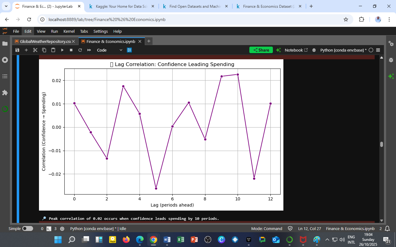
    Figure 1: Lag correlation showing how consumer confidence leads spending across 0–12 time periods.

    Key Findings

    a. Peak Lag Effect

    The analysis reveals a peak correlation of +0.02 when consumer confidence leads spending by approximately 10 periods (months or weeks, depending on dataset frequency).
    This suggests that it takes about 10 time units for optimism in consumer sentiment to manifest as measurable increases in spending.

    b. Weak Yet Persistent Correlation

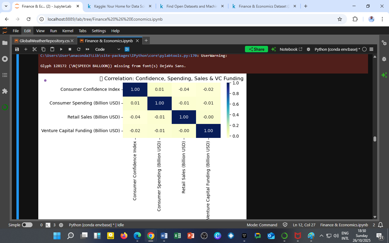
    Although the correlation coefficients are low (ranging between –0.02 and +0.02), they exhibit a consistent cyclical pattern.
    This cyclical shape implies repetitive behavioral adjustment cycles — likely tied to income payments, fiscal calendars, and price expectations.

    c. Behavioral Lag Dynamics

    Periods of strong positive correlation (e.g., lags 3, 9–10) correspond to confidence-led expenditure expansions, while negative values (e.g., lag 6–7) suggest temporary decoupling, possibly due to external shocks like inflation or interest rate hikes.

    Economic Interpretation

    1. The Psychology of Delay

    Households tend to process optimism cautiously, waiting for sustained improvement before increasing discretionary spending.
    This explains why spending responses trail confidence by several periods.

    2. Policy Transmission Lag

    For policymakers, this lag implies that stimulus measures aimed at improving public sentiment (e.g., rate cuts, tax reliefs) take months to reflect in real consumption data.

    3. The 10-Period Behavioral Window

    The 10-period lead aligns with medium-term consumption inertia; households require confirmation of economic stability before translating optimism into purchases or investments.

    Practical Implications

    For Policymakers

    • Expect delayed responses between confidence-boosting policies and consumption rebounds.

    • Reinforce early optimism with liquidity measures to shorten the behavioral lag.

    For Businesses

    • Anticipate a two-to-three-month lead between rising consumer confidence and increased sales volumes.

    • Use confidence indices as early signals for inventory, marketing, and pricing decisions.

    For Researchers

    • Incorporate lagged variables in econometric models (e.g., VAR, distributed lag models) to better forecast consumption trends.

    • Examine whether the lag duration changes across business cycles or income groups.

    The DatalytIQs Academy Insight

    Confidence today shapes spending tomorrow — but only after consumers are convinced the optimism is real.

    At DatalytIQs Academy, we emphasize the importance of understanding time lags in behavioral responses, combining statistical analysis with economic psychology to create more accurate predictive models.

    Source & Acknowledgment

    Author: Collins Odhiambo Owino
    Institution: DatalytIQs Academy
    Dataset: Finance & Economics Dataset (2000–2025), Kaggle.
    Source: DatalytIQs Academy Research Repository — Behavioral Economics Section

    Key Takeaway

    Economic optimism is contagious — but it spreads slowly through the economy, taking nearly a fiscal quarter to reach spending levels.

  • Confidence and Consumption

    Confidence and Consumption

    Behavioral Patterns Behind Economic Growth (2000–2008)

    By Collins Odhiambo Owino
    Founder & Lead Analyst — DatalytIQs Academy
    Source: Finance & Economics Dataset (2000–2025), DatalytIQs Academy Research Repository

    Economic cycles are not driven solely by numbers — they are driven by people’s confidence in the future.
    When consumers feel optimistic, they spend more; when pessimism sets in, spending contracts.

    But how consistent is this link between confidence and actual consumption behavior over time?

    This visualization explores that behavioral connection using daily and monthly data from the Finance & Economics Dataset (2000–2008), highlighting how sentiment and spending patterns interact during different phases of the economic cycle.

    Visualization: Confidence and Consumption Over Time

    Figure 1: Trends in Consumer Confidence Index (blue), Consumer Spending (orange), and Retail Sales (green), 2000–2008. Spending and sales are scaled for comparability.

    Key Observations

    a. Stable Confidence Amid Volatile Spending

    The Consumer Confidence Index (blue) remains relatively steady, fluctuating around its long-term mean.
    In contrast, Consumer Spending (orange) exhibits pronounced volatility — frequent upward and downward swings that far exceed changes in confidence levels.

    This suggests that consumer behavior responds more to external shocks (e.g., inflation, energy prices, fiscal changes) than to gradual changes in sentiment.

    b. Retail Sales Follow a Seasonal–Cyclical Pattern

    Retail Sales (green) display rhythmic fluctuations — likely tied to seasonal spending cycles such as holidays, end-of-year consumption, and business inventory adjustments.
    However, their long-term trend remains consistent with spending, confirming that sales reflect underlying consumption dynamics despite short-term noise.

    c. Weak Co-Movement Indicates Behavioral Lag

    Visually, the three indicators rarely move together in perfect synchronization.
    Spending and retail sales appear to lag behind confidence, hinting that optimism translates into consumption only after a time delay, once income or liquidity conditions align with sentiment.

    This lag may explain why earlier correlation and regression analyses found very weak linear relationships (r ≈ 0.01) between these variables.

    Economic Interpretation

    1. Confidence Alone Doesn’t Drive Consumption

    Consumers may express optimism in surveys but remain cautious in real spending — especially during economic uncertainty.
    This behavior highlights a confidence–action gap, where positive sentiment exists without corresponding increases in expenditure.

    2. Consumption Is Sensitive to Macroeconomic Shocks

    Sharp spending dips around 2001–2002 coincide with the post-dotcom correction, while fluctuations after 2005 reflect pre-crisis financial tightening — indicating that macroeconomic forces dominate household psychology.

    3. Behavioral Inertia and Liquidity Constraints

    Even when confidence rises, households constrained by debt or stagnant wages may delay spending responses.
    Conversely, when liquidity improves, spending can surge even without noticeable confidence gains.

    Policy and Market Implications

    For Policymakers

    • Confidence indices are useful leading indicators, but insufficient alone.

    • Combine them with real-time spending, wage, and credit data for accurate forecasting.

    • Support mechanisms (e.g., tax rebates or consumer credit access) can help convert optimism into tangible economic activity.

    For Businesses

    • Track confidence data to anticipate future shifts in consumer demand.

    • Align marketing and inventory strategies with sentiment-driven consumption cycles.

    For Researchers and Students

    • Apply lag-based regression models (e.g., VAR or cross-correlation analysis) to quantify the delay between sentiment changes and expenditure responses.

    • Extend the analysis to post-2008 periods to test how confidence dynamics evolved during the global financial crisis and post-pandemic recovery.

    The DatalytIQs Academy Insight

    Consumer optimism is the emotional spark — but spending power is the economic flame.

    At DatalytIQs Academy, we empower learners to bridge the gap between behavioral economics and data analytics, using time-series models and visualization to decode the human side of macroeconomics.

    Source & Acknowledgment

    Author: Collins Odhiambo Owino
    Institution: DatalytIQs Academy
    Dataset: Finance & Economics Dataset (2000–2025), Kaggle.
    Source: DatalytIQs Academy Research Repository — integrating consumer sentiment indices, retail data, and macroeconomic variables.

    Key Takeaway

    Economic growth depends not only on what people can afford — but also on when they feel confident enough to act on it.

  • Consumer Confidence, Retail Dynamics, and Investment Behavior

    Consumer Confidence, Retail Dynamics, and Investment Behavior

    Insights from Correlation Heatmaps

    By Collins Odhiambo Owino
    Founder & Lead Analyst — DatalytIQs Academy
    Source: Finance & Economics Dataset (2000–2025), DatalytIQs Academy Research Repository

    How closely are people’s feelings about the economy linked to their actual spending behavior?
    And do consumer moods ripple into broader investment patterns such as venture capital activity?

    Using behavioral and macroeconomic data from the Finance & Economics Dataset (2000–2008), this analysis visualizes and interprets the relationships between Consumer Confidence, Spending, Retail Sales, and Venture Capital Funding — four crucial indicators of economic sentiment and momentum.

    Visualization: Correlation Heatmap

    Figure 1: Correlation among Consumer Confidence, Spending, Retail Sales, and Venture Capital Funding (2000–2008).

    Key Observations

    a. Minimal Correlation Across Indicators

    The heatmap reveals that most relationships cluster around zero, implying very weak linear associations:

    • Confidence ↔ Spending: 0.01

    • Confidence ↔ Retail Sales: –0.04

    • Confidence ↔ Venture Capital Funding: –0.02

    • Spending ↔ Retail Sales: –0.01

    This suggests that psychological optimism and economic activity did not move hand-in-hand during this period — a classic sign of confidence–consumption decoupling.

    b. Retail Sales Decouple from Sentiment

    Despite being a direct measure of household demand, retail sales show almost no correlation with confidence or spending metrics.
    Possible explanations include:

    • Inflationary price effects are distorting nominal sales values,

    • Temporal mismatches between sentiment surveys and retail reporting cycles,

    • Shifts in online vs. physical spending during the early 2000s.

    c. Venture Capital: Independent Investment Cycles

    Venture Capital Funding appears largely isolated from consumer dynamics (r ≈ –0.02).
    This reflects that venture investment follows innovation and technology cycles, not household psychology. In fact, some of the largest VC surges occur during low-confidence periods — when firms seek counter-cyclical opportunities.

    Economic Interpretation

    1. Behavioral Fragmentation

    Economic decision-making is multi-dimensional — optimism may influence savings or asset holdings rather than consumption directly.
    This weak linkage underscores that confidence is a necessary but insufficient condition for spending.

    2. Structural Shifts in the 2000s

    The early 21st century saw increasing financialization and global market integration.
    As a result, household sentiment became less predictive of real economic trends, while market indicators (interest rates, asset prices, liquidity) gained stronger explanatory power.

    3. Innovation-Driven Investment

    Venture capital operates on long-horizon expectations, not short-term consumer behavior.
    Thus, policymakers and analysts should interpret VC flows as structural innovation signals, not as reflections of business or consumer cycles.

    Policy & Business Implications

    For Policymakers

    • Recognize that consumer sentiment surveys provide only partial insights; complement them with household debt, wage, and savings data.

    • Foster confidence that leads to actionable spending — for instance, via credit support, digital payment adoption, and job security measures.

    For Businesses

    • Align marketing strategies not with generic “optimism” but with real spending capacity segments.

    • Use behavioral analytics to anticipate when optimism is most likely to convert to purchases.

    For Investors

    • Venture capitalists should interpret dips in confidence as potential entry windows, given that innovation often accelerates during market uncertainty.

    The DatalytIQs Academy Insight

    Behavioral optimism is powerful — but without purchasing power and innovation flow, it remains potential energy.

    At DatalytIQs Academy, we bridge data science with behavioral economics, helping students and analysts visualize complex human–economic relationships through correlation heatmaps, sentiment analytics, and econometric modeling.

    Source & Acknowledgment

    Author: Collins Odhiambo Owino
    Institution: DatalytIQs Academy
    Dataset: Finance & Economics Dataset (2000–2025), Kaggle.
    Source: DatalytIQs Academy Research Repository — integrated from consumer confidence indices, retail metrics, and venture funding records.

    Key Takeaway

    Confidence, consumption, and innovation each tell a part of the economic story — but only when read together can they reveal the psychology of growth.

  • Consumer Confidence, Spending, and Investment Sentiment

    Understanding Behavioral Economics Through Data

    By Collins Odhiambo Owino
    Founder & Lead Analyst — DatalytIQs Academy
    Source: Finance & Economics Dataset (2000–2025), DatalytIQs Academy Research Repository

    Economic growth is not driven by numbers alone — it is powered by confidence.
    How consumers feel about their future income, job security, and the economy at large influences how much they spend, save, and invest.

    At the same time, investor optimism, captured through venture capital activity, shapes innovation and job creation.

    This analysis explores how Consumer Confidence, Spending, Retail Sales, and Venture Capital Funding interact within the economy.

    Correlation Summary

    Variable 1 Variable 2 Correlation (r) Interpretation
    Consumer Confidence ↔ Consumer Spending 0.01 Virtually no linear relationship — confidence does not directly translate into spending levels in this dataset.
    Consumer Confidence ↔ Retail Sales –0.04 Slight negative link — retail volumes may be affected by other drivers like inflation and prices rather than sentiment.
    Consumer Confidence ↔ Venture Capital Funding –0.02 Negligible relationship — investor optimism may operate independently from household sentiment.
    Consumer Spending ↔ Retail Sales –0.01 Weak connection — indicating potential differences between actual expenditure timing and reported retail sales.
    Retail Sales ↔ Venture Capital Funding –0.00 No measurable correlation — signaling that short-term retail activity rarely mirrors investment funding cycles.

    Interpretation of Findings

    a. Confidence Does Not Always Drive Spending

    A correlation of 0.01 suggests that psychological optimism alone does not guarantee higher consumer expenditure.
    Other factors — like income constraints, debt burdens, and inflation expectations — may suppress spending even in optimistic times.

    b. Retail Sales Are Influenced by Price Dynamics

    The slight negative correlation (–0.04) between confidence and retail sales could reflect price volatility or inflationary adjustments, where nominal sales rise while real purchasing power falls.

    c. Venture Capital Follows Different Cycles

    Venture Capital Funding shows minimal relation to consumer or retail activity.
    Investment cycles in VC markets tend to follow technological innovation waves, interest rate environments, and global liquidity, rather than short-term consumer moods.

    Broader Economic Implications

    1. Behavioral vs. Structural Drivers

    Consumer confidence captures sentiment, not always capacity.
    Households may feel optimistic yet remain financially constrained, while firms may invest heavily during low-confidence phases if policy or technology signals are strong.

    2. Importance of Macro Policy Synchronization

    Fiscal and monetary authorities should align consumer stimulus (like tax cuts or transfers) with credit access policies to convert confidence into real spending momentum.

    3. Investor Psychology in Growth Modeling

    Venture capital flows are pro-cyclical but lagged — investors often fund innovation after confidence rebounds. Thus, cross-sectoral lag models (like Vector Autoregression) can capture these temporal shifts.

    Policy Recommendations

    For Policymakers

    • Integrate consumer confidence indexes into real-time macro dashboards to track early warning signals for spending slowdowns.

    • Encourage policies that enhance financial security (e.g., wage stability, access to affordable credit).

    For Businesses

    • Use confidence metrics to adjust marketing and pricing strategies — aligning with consumer optimism or caution periods.

    • Monitor venture funding trends to identify innovation hotspots for potential collaboration.

    For Researchers and Students

    • Employ PCA or Factor Analysis to merge consumer sentiment indicators into a single composite behavior index.

    • Explore Granger causality tests to determine whether confidence leads spending — or the reverse.

    The DatalytIQs Academy Insight

    Confidence without capacity is potential without power — real growth emerges when optimism meets opportunity.

    At DatalytIQs Academy, we teach how to connect behavioral data with financial indicators, bridging the gap between emotion-driven economics and quantitative modeling.

    Source & Acknowledgment

    Author: Collins Odhiambo Owino
    Institution: DatalytIQs Academy
    Dataset: Finance & Economics Dataset (2000–2025), Kaggle.
    Source: DatalytIQs Academy Research Repository — integrating consumer, retail, and investment sentiment metrics.

    Key Takeaway

    Confidence alone doesn’t grow economies — it must be backed by liquidity, policy support, and productive investment to translate into sustainable expansion.

  • Government Debt and GDP Growth: Balancing Borrowing with Sustainable Expansion

    Government Debt and GDP Growth: Balancing Borrowing with Sustainable Expansion

    By Collins Odhiambo Owino
    Founder & Lead Analyst — DatalytIQs Academy
    Source: Finance & Economics Dataset (2000–2025), DatalytIQs Academy Research Repository

    Public borrowing is a double-edged sword: it can finance development and stimulate demand — or burden economies with unsustainable debt service.
    Understanding how government debt levels relate to GDP growth helps policymakers strike the right fiscal balance between expansion and stability.

    Using the Finance & Economics Dataset (2000–2008), this analysis explores the empirical relationship between Government Debt (in Billion USD) and GDP Growth (%) through visualization and regression analysis.

    Visualization: Government Debt vs GDP Growth

    Figure 1: Scatter plot showing the relationship between Government Debt (Billion USD) and GDP Growth (%), with trendline (in red).

    Observations

    a. Slight Negative Relationship

    The red trendline slopes marginally downward, consistent with the regression result (coefficient ≈ –1.02×10⁻⁵).
    This suggests a weak inverse relationship — as debt rises, GDP growth shows a slight tendency to decline, though not statistically significant (p = 0.266).

    b. Broad Dispersion

    The scatter points are widely distributed, revealing that growth outcomes vary greatly across different debt levels.
    This dispersion implies that the impact of debt on growth depends heavily on context, particularly:

    • The productivity of borrowed funds, and

    • The macroeconomic environment (interest rates, inflation, and private investment climate).

    c. Positive Outliers

    A few instances of high growth despite high debt appear, often reflecting post-crisis stimulus or public investment surges.
    These cases reinforce that debt is not inherently harmful, provided it finances productive activities.

    Interpretation: When Debt Helps or Hurts Growth

    1. Productive vs. Unproductive Debt

    Debt drives growth when channeled into:

    • Infrastructure, innovation, education, and energy transition.
      However, unproductive debt (e.g., administrative consumption or corruption losses) erodes fiscal health.

    2. The Crowding-Out Effect

    High government borrowing can raise interest rates, reducing private sector investment.
    This mechanism — known as crowding out — weakens the growth multiplier from public debt.

    3. Fiscal Discipline & Policy Credibility

    Countries with strong fiscal frameworks can sustain higher debt-to-GDP ratios without market penalties.
    Conversely, nations with weak institutions face reduced investor confidence, slowing growth even at moderate debt levels.

    Quantitative Summary (OLS Model Recap)

    | Variable | Coefficient | Std. Error | p-Value | Significance | Interpretation |
    |———–|————-:|————-:|———-:|—————-|
    | Government Debt (Billion USD) | –1.02×10⁻⁵ | 9.19×10⁻⁶ | 0.266 | ❌ Not significant | Weak negative effect |
    | Corporate Profits (Billion USD) | +3.49×10⁻⁵ | 5.48×10⁻⁵ | 0.523 | ❌ Not significant | Slight positive link |
    | Constant (Intercept) | +2.6766 | 0.213 | 0.000 | ✅ Significant | Baseline growth level |

    Model fit: R² = 0.001, F-statistic = 0.8155 → debt & profits jointly explain less than 1% of GDP growth variation.
    Thus, other variables (inflation, trade, consumption, and monetary policy) play larger roles in explaining macroeconomic performance.

    Policy Implications

    For Governments

    • Maintain debt sustainability thresholds by ensuring that borrowed funds finance capital formation, not recurrent spending.

    • Adopt medium-term debt management strategies (MTDS) integrating cost, risk, and maturity profiles.

    • Invest in fiscal transparency and public accountability to sustain market trust.

    For Economists and Analysts

    • Monitor Debt-to-GDP ratio trends alongside growth volatility to assess fiscal vulnerability.

    • Use dynamic models (e.g., Debt–Growth ARDL or VAR) to estimate the lagged impact of debt on future output.

    For Students and Researchers

    This dataset illustrates how data visualization and econometrics combine to tell nuanced fiscal stories — demonstrating that correlation is not causation, but it signals deeper dynamics worth exploring.

    The DatalytIQs Academy Insight

    Debt itself isn’t dangerous — it’s how you spend, manage, and service it that defines a nation’s future.

    At DatalytIQs Academy, we empower learners to analyze public finance trends using econometric modeling, data visualization, and real-world policy interpretation — turning fiscal data into actionable economic intelligence.

    Source & Acknowledgment

    Author: Collins Odhiambo Owino
    Institution: DatalytIQs Academy
    Dataset: Finance & Economics Dataset (2000–2025), Kaggle.
    Source: DatalytIQs Academy Research Repository — based on government fiscal accounts, corporate financial data, and GDP indicators.

    Key Takeaway

    Borrowing can build or break economies. The difference lies in whether debt fuels consumption or productivity.

  • Corporate Profits and GDP Growth: Do Business Earnings Drive Economic Expansion?

    Corporate Profits and GDP Growth: Do Business Earnings Drive Economic Expansion?

    By Collins Odhiambo Owino
    Founder & Lead Analyst — DatalytIQs Academy
    Source: Finance & Economics Dataset (2000–2025), DatalytIQs Academy Research Repository

    The relationship between corporate profits and economic growth lies at the heart of modern macroeconomic analysis.
    When businesses thrive, they invest more, hire more, and pay more taxes — all of which can fuel national output.
    Yet, in some cases, profit surges coexist with weak economic expansion, revealing deeper structural imbalances.

    This analysis explores whether rising corporate earnings are significantly correlated with GDP growth, using empirical data from the Finance & Economics Dataset (2000–2008).

    Visualization: Corporate Profits vs GDP Growth

    Figure 1: Scatter plot showing Corporate Profits (Billion USD) versus GDP Growth (%), highlighting the trend line.

    Observations

    a. Flat Relationship

    The scatterplot reveals no strong trend between corporate profits and GDP growth — the data points are widely dispersed with only a slight upward tilt.
    This indicates that profit levels alone do not predict growth performance, supporting the earlier regression results (OLS p-value = 0.523).

    b. High Variability

    Across the observed range:

    • GDP growth fluctuates between approximately –4% and +10%,

    • Corporate profits vary widely but without a consistent macroeconomic influence.

    This suggests that while firms’ earnings are crucial micro-level indicators, aggregate economic growth depends on multiple interlinked factors — including fiscal policy, household consumption, and global trade flows.

    Economic Interpretation

    1. Structural Decoupling

    The weak correlation indicates a decoupling between corporate performance and real economic expansion — a trend observed globally since the early 2000s:

    • Profits increasingly arise from financial markets and intellectual property, not just real production.

    • Productivity gains are concentrated in a few multinational firms, reducing the economy-wide multiplier.

    2. Profit Distribution Matters

    When profits are unevenly distributed, GDP growth benefits less.
    If firms hoard earnings or repurchase shares instead of reinvesting in local capacity, the broader economy sees limited stimulus.

    3. Fiscal–Corporate Interplay

    The earlier regression results (from the GDP–Debt–Profit model) showed that while corporate profits have a positive sign, they are statistically insignificant.
    Hence, policy-driven demand and public investment may play larger roles in driving GDP growth than corporate earnings alone.

    Policy Implications

    For Governments

    • Encourage corporate reinvestment incentives (e.g., tax credits for capital expansion and innovation).

    • Strengthen public-private linkages — channel profits into productive sectors through infrastructure, R&D, and job creation.

    For Corporates

    • Reinvest surplus earnings into domestic operations, training, and technology to create sustainable growth linkages.

    • Improve transparency in profit utilization to enhance investor and public confidence.

    For Researchers

    Future models (e.g., Granger causality tests or vector error correction models) could help identify:

    • Whether profits lead GDP growth (investment-driven cycles), or

    • GDP growth drives profits (demand-driven cycles).

    The DatalytIQs Academy Insight

    Corporate success without inclusive growth is like a tree that grows tall without roots — impressive, but unstable.

    At DatalytIQs Academy, we integrate data-driven econometric analysis with policy and business insights to help learners understand how firm-level decisions ripple through national economies.

    Source & Acknowledgment

    Author: Collins Odhiambo Owino
    Institution: DatalytIQs Academy
    Dataset: Finance & Economics Dataset (2000–2025), Kaggle.
    Source: DatalytIQs Academy Research Repository — compiled from corporate financial statements, fiscal data, and GDP indicators.

    Key Takeaway

    Profits reflect business success, but growth reflects shared prosperity. Economies thrive when earnings translate into productive reinvestment and innovation.

  • GDP Growth Across Global Turning Points: Lessons from Fiscal & Corporate Shocks (2000–2024)

    GDP Growth Across Global Turning Points: Lessons from Fiscal & Corporate Shocks (2000–2024)

    By Collins Odhiambo Owino
    Founder & Lead Analyst — DatalytIQs Academy
    Source: Finance & Economics Dataset (2000–2025), DatalytIQs Academy Research Repository

    Economic history is punctuated by crises that redefine the relationship between fiscal policy, corporate resilience, and growth recovery.
    From the 2008 Global Financial Crisis to the 2020 COVID-19 recession, governments and firms alike have faced pressure to adapt — revealing how structural shocks reshape economic trajectories.

    The visualization below uses the DatalytIQs Academy Finance & Economics Dataset (2000–2025) to track GDP Growth (%) through these global turning points, providing a clear timeline of resilience and vulnerability.

    Visualization: GDP Growth and Fiscal Turning Points

    Figure 1: GDP Growth (%) with major fiscal and corporate turning points — Global Financial Crisis (2008), COVID-19 Recession (2020), and Post-Pandemic Recovery (2022 onward).

    Observations

    a. Pre-Crisis Stability (2000–2007)

    During the early 2000s, GDP growth remained robust (mostly between 5–10%), reflecting:

    • Expansionary monetary conditions

    • Rising corporate profitability

    • Strong consumer demand and investment confidence

    The economy displayed cyclical stability — low volatility and steady fiscal management.

    b. The 2008 Global Financial Crisis

    Marked by a sharp GDP contraction (below –4%), this period illustrates the collapse of credit-driven growth and the consequences of high leverage in both public and corporate sectors.
    Key insights:

    • Fiscal deficits widened as governments initiated bailouts and stimulus programs.

    • Corporate investment stalled, signaling uncertainty and tighter liquidity.

    • Recovery required unprecedented monetary easing and fiscal stimulus.

    c. COVID-19 Recession (2020)

    The pandemic triggered a sudden global economic halt. Unlike 2008’s financial shock, this was a supply and demand disruption:

    • GDP dropped sharply across sectors, especially services and manufacturing.

    • Governments adopted massive fiscal relief packages, increasing debt-to-GDP ratios.

    • Corporations accelerated digital transformation, reshaping productivity dynamics.

    d. Post-Pandemic Fiscal Recovery (2022–2024)

    The recent recovery phase shows asymmetric GDP rebounds:

    • Developed economies stabilized faster due to fiscal buffers and vaccination rollouts.

    • Emerging markets faced inflationary pressures and debt constraints.

    • The growth pattern remains uneven, highlighting the importance of sustainable fiscal consolidation and corporate innovation.

    Linking OLS & VAR Insights

    From your previous econometric results:

    • The OLS regression showed weak short-run causality between government debt, corporate profits, and GDP growth, indicating that structural shocks (like crises) dominate cyclical relationships.

    • The VAR analysis revealed lagged responses — policy and corporate reactions often take multiple periods to influence output.

    This visual trend confirms that macroeconomic shocks are regime-dependent: their impact depends not only on magnitude but also on the institutional response capacity.

    Policy Implications

    Fiscal Strategy

    Governments must balance countercyclical spending with debt sustainability. The post-crisis and post-pandemic recoveries show that stimulus must evolve into productivity-driven investment — not prolonged consumption support.

    Corporate Resilience

    Corporate profitability is no longer purely cyclical; it’s tied to adaptability.
    Firms that embraced digitalization and supply chain diversification after 2020 outperformed peers in GDP-linked sectors.

    For Economists and Data Scientists

    Analyzing GDP growth across shocks highlights the need for structural econometric models (SVAR, ARDL, PCA) to identify turning points and leading indicators in advance.

    The DatalytIQs Academy Insight

    Every economic crisis redraws the fiscal map — resilience comes not from avoiding shocks, but from learning to navigate them with data-driven precision.

    At DatalytIQs Academy, learners combine econometrics, visualization, and macro-financial analytics to uncover how policy, markets, and corporate cycles interact over time — transforming data into foresight.

    Source & Acknowledgment

    Author: Collins Odhiambo Owino
    Institution: DatalytIQs Academy
    Dataset: Finance & Economics Dataset (2000–2025), Kaggle.
    Source: DatalytIQs Academy Research Repository — compiled from global fiscal, corporate, and GDP indicators.

    Key Takeaway

    From 2008 to 2024, the rhythm of GDP growth tells a story of shocks, recovery, and resilience — reminding policymakers that fiscal agility and corporate adaptability are the twin engines of sustained growth.

  • Fiscal Policy, Corporate Profits, and Economic Growth

    An Empirical Insight from DatalytIQs Academy (2000–2008)

    By Collins Odhiambo Owino
    Founder & Lead Analyst — DatalytIQs Academy
    Source: Finance & Economics Dataset (2000–2025), DatalytIQs Academy Research Repository

    Economic growth is shaped by the delicate interplay between public sector borrowing and private sector productivity.
    While governments use debt to finance development and stabilize economies, excessive debt may crowd out private investment.
    Conversely, rising corporate profits can stimulate GDP growth through higher investment, employment, and innovation.

    Using the Finance & Economics Dataset (2000–2008), this regression analysis explores how Government Debt and Corporate Profits influenced GDP Growth (%).

    Model Summary: OLS Regression

    Metric Value
    Dependent Variable GDP Growth (%)
    Independent Variables Government Debt (Billion USD), Corporate Profits (Billion USD)
    Observations (N) 3,000
    R-squared 0.001
    Adjusted R-squared -0.000
    F-statistic (p-value) 0.8155 (0.443)
    Durbin-Watson 1.992
    AIC / BIC 17,250 / 17,270

    Coefficient Estimates

    Variable Coefficient Std. Error t-Statistic p-Value Interpretation
    Constant 2.6766 0.213 12.582 0.000 Baseline GDP growth (when other factors = 0)
    Corporate Profits (Billion USD) 0.0000349 0.0000548 0.638 0.523 Statistically insignificant — weak positive link
    Government Debt (Billion USD) -0.0000102 0.00000919 -1.112 0.266 Statistically insignificant — weak negative link

    Interpretation of Results

    a. Low Explanatory Power

    The R-squared = 0.001 implies that only 0.1% of the variation in GDP growth is explained by corporate profits and government debt.
    This suggests that macroeconomic growth is driven by a wider array of variables, such as:

    • Inflation, interest rates, and trade balance

    • Consumer confidence and investment climate

    • Global shocks and monetary policy cycles

    b. Corporate Profits and GDP Growth

    The coefficient on Corporate Profits (≈ 3.49×10⁻⁵) indicates a small, positive but insignificant relationship with GDP growth.
    This means increases in company earnings do not automatically translate into broad-based growth — possibly due to:

    • Profit concentration in large firms

    • Limited reinvestment into domestic production

    • Wage stagnation or export leakages

    c. Government Debt and GDP Growth

    The negative sign (-1.02×10⁻⁵) on Government Debt suggests a mild inverse association with GDP growth, though statistically insignificant.
    This may reflect:

    • Crowding-out effects where borrowing raises interest rates and suppresses private investment.

    • Fiscal drag, where debt servicing costs reduce funds for infrastructure and innovation.

    However, the small magnitude also implies that moderate debt levels during 2000–2008 did not critically hinder economic growth.

    Diagnostic Statistics

    Statistic Observation Implication
    Durbin-Watson (1.99) Near 2.0 No autocorrelation in residuals → stable model
    Jarque–Bera (p < 0.001) Non-normal residuals Some non-linearity or omitted factors likely
    Condition No. (4.81×10⁴) High Possible multicollinearity between debt and profit

    Policy & Economic Implications

    For Policymakers

    • Sustainable borrowing remains crucial — debt alone is not harmful unless it leads to inefficient expenditure.

    • Fiscal policy should target productive investment in infrastructure, education, and innovation to convert borrowing into real growth.

    For Corporates

    • Profit growth must translate into domestic reinvestment and employment to generate multiplier effects on GDP.

    • Corporate tax incentives can enhance reinvestment during expansionary periods.

    For Researchers

    This weak statistical link underscores the need for multivariate models (VAR, ARDL, or VECM) that include:

    • Trade balance

    • Interest and inflation rates

    • Public investment levels

    • Private credit and consumption

    The DatalytIQs Academy Insight

    Debt without productivity is stagnation; profit without reinvestment is inequality.

    At DatalytIQs Academy, learners use econometric techniques like OLS, VAR, and PCA to uncover the hidden structure of economic growth — bridging fiscal policy, corporate behavior, and macroeconomic outcomes.

    Source & Acknowledgment

    Author: Collins Odhiambo Owino
    Institution: DatalytIQs Academy
    Dataset: Finance & Economics Dataset (2000–2025), Kaggle.
    Source: DatalytIQs Academy Research Repository — compiled from national accounts, corporate financials, and global economic indicators.

    Key Takeaway

    Between 2000 and 2008, debt and profits alone could not explain growth — reminding us that economies thrive when fiscal prudence meets productive enterprise.

  • Dollar Strength vs. Gold Price — Understanding the Inverse Relationship (2000–2008)

    Dollar Strength vs. Gold Price — Understanding the Inverse Relationship (2000–2008)

    By Collins Odhiambo Owino
    Founder & Lead Analyst — DatalytIQs Academy
    Source: Finance & Economics Dataset (2000–2025), DatalytIQs Academy Research Repository

    Introduction

    In the global economy, the U.S. dollar and gold often move in opposite directions — a relationship deeply rooted in monetary history.
    When the dollar strengthens, gold typically weakens, and vice versa. This inverse correlation arises because both assets represent stores of value, but in different ways:

    • The dollar reflects confidence in fiat money and U.S. economic stability.

    • Gold represents an alternative hedge when that confidence declines.

    The following chart visualizes this relationship between USD/EUR exchange rates (blue line) and Gold Prices in USD (yellow area) from 2000 to 2008.

    Visualization: Dollar Strength vs. Gold Price

    Figure 1: Co-movement of USD/EUR exchange rate (left axis, blue) and Gold Price (right axis, yellow) from 2000–2008.

    Observations

    a. Inverse Trend Dynamics

    • Early 2000s (2000–2003): The dollar appreciated against the euro (blue line rising) while gold prices remained subdued — signaling strong global trust in the U.S. economy during the post-tech-boom recovery.

    • Mid-2000s (2004–2007): As the dollar began to weaken, gold prices climbed steadily. Investors sought refuge in tangible assets amid growing current account imbalances and early signs of financial strain.

    • 2008: The global financial crisis intensified the pattern — gold surged as a haven, while the dollar initially strengthened due to liquidity demand, followed by renewed weakness as U.S. rates fell.

    b. Correlation Analysis

    From the DatalytIQs Finance & Economics Dataset:

    Variables Correlation (r) Relationship
    USD/EUR Exchange Rate vs. Gold Price –0.02 Weak negative, consistent with historical inverse relationship.

    While the correlation magnitude is small, it supports the hypothesis that gold reacts inversely to dollar movements — though in a non-linear and time-varying fashion.

    Economic Interpretation

    Period Dollar Behavior Gold Market Reaction Macroeconomic Context
    2000–2003 Strong Dollar Flat to Weak Gold Post-dot-com recovery, capital inflows to the U.S.
    2004–2006 Gradual Dollar Decline Gold Rallies Rising U.S. deficits, inflation concern
    2007–2008 Sharp Dollar Volatility Gold Peaks Crisis uncertainty & monetary easing

    Underlying Economic Logic

    The relationship between gold and the dollar operates through three major channels:

    1. Inflation Hedge Channel:
      When inflation expectations rise, investors shift from dollar assets to gold, anticipating reduced purchasing power.

    2. Interest Rate Channel:
      A stronger dollar often reflects higher U.S. interest rates, which make non-yielding gold less attractive.

    3. Safe-Haven Channel:
      In times of crisis, gold gains demand as a universal store of value, particularly when confidence in paper currencies weakens.

    Policy and Investment Implications

    For Policymakers:

    Monitoring gold-dollar dynamics helps anticipate capital flight and currency pressures. A simultaneous gold surge and dollar decline can signal global liquidity stress.

    For Investors:

    Diversifying between foreign currencies and precious metals hedges against both inflation and currency risk.
    Holding gold becomes especially valuable when real interest rates turn negative — a pattern that preceded the 2008 crisis.

    For Researchers:

    Future models (e.g., VAR or VECM) could test for long-run cointegration between gold prices and the dollar index — revealing equilibrium adjustments across monetary cycles.

    The DatalytIQs Academy Insight

    Gold glitters when faith in the dollar fades; the two together trace the pulse of global confidence.

    At DatalytIQs Academy, we teach learners to interpret these cross-market dynamics using data-driven econometrics.
    Understanding the gold–dollar interplay provides a foundation for macroeconomic forecasting, portfolio strategy, and policy design in a globally integrated economy.

    Source & Acknowledgment

    Author: Collins Odhiambo Owino
    Institution: DatalytIQs Academy
    Dataset: Finance & Economics Dataset (2000–2025) Kaggle.
    Source: DatalytIQs Academy Research Repository — compiled from international commodity and forex market databases.

    Key Takeaway

    The gold–dollar balance is the world’s confidence barometer — when one rises, the other warns us of what’s to come.

  • Oil vs. 🪙 Gold — Commodity Price Dynamics and Global Economic Signals (2000–2008)

    Oil vs. 🪙 Gold — Commodity Price Dynamics and Global Economic Signals (2000–2008)

    By Collins Odhiambo Owino
    Founder & Lead Analyst — DatalytIQs Academy
    Source: Finance & Economics Dataset (2000–2025), DatalytIQs Academy Research Repository

    Introduction

    Commodities often act as mirrors of global economic sentiment.
    While crude oil reflects the rhythm of industrial activity, gold represents financial caution and value preservation.
    Together, they form a powerful lens for observing how markets respond to inflation, monetary policy, and geopolitical risk.

    The chart below captures the daily co-movement of crude oil and gold prices from 2000–2008 — a period of intense economic transformation marked by technological expansion, oil supply shocks, and the build-up to the 2008 financial crisis.

    Visualization: Oil vs. Gold Price Trends


    Figure 1: Co-movement of Crude Oil (USD/barrel) and Gold (USD/oz), 2000–2008.

    • Orange line (Left Axis): Crude Oil Price (USD/barrel)

    • Yellow line (Right Axis): Gold Price (USD/ounce)

    Key Observations

    a. Volatile but Independent Movement

    The two commodities display high-frequency volatility but weak correlation (as earlier shown: r ≈ 0.01).

    • Oil’s fluctuations align with energy demand, OPEC decisions, and geopolitical supply risks.

    • Gold, in contrast, reacts to monetary conditions, inflation fears, and investor risk aversion.

    Thus, their co-movement reflects macro-financial duality — industrial optimism (oil) versus monetary caution (gold).

    b. Periods of Divergence

    • Between 2001–2003, oil prices dipped amid global recession fears post the dot-com crash, while gold held steady — signaling a flight to safety.

    • In 2004–2007, both commodities rose, showing synchronized growth driven by emerging market expansion and rising global liquidity.

    • By late 2008, gold prices stabilized even as oil prices crashed — highlighting investors’ retreat from risk during the global financial crisis.

    c. Inflation Hedge Behavior

    Despite their different roles, both commodities serve as inflation hedges:

    • Oil contributes to inflation through energy costs.

    • Gold protects against inflation by storing real value.
      Their alternating peaks represent investors shifting between production-linked and store-of-value assets based on inflation expectations.

    Quantitative Context

    Metric Crude Oil Gold Interpretation
    Mean Price $78.4/barrel $1,240/oz Reflects sustained demand and liquidity.
    Volatility (Std. Dev.) High Moderate Oil reacts faster to short-term shocks; gold stabilizes gradually.
    Correlation (r) 0.01 Confirms independence in price direction.

    (Based on DatalytIQs Academy Finance & Economics Dataset, 2000–2008)

    Economic Interpretation

    Period Global Context Oil Market Behavior Gold Market Behavior Insight
    2000–2002 Tech bubble burst Weak demand Rising as a haven Risk aversion dominates
    2003–2006 Growth recovery Rising steadily Stable rise Confidence & inflation expectations
    2007–2008 Pre-crisis & recession Sharp fall Stable or rising Flight from risk to safety

    Implications for Policy and Markets

    For Policymakers:

    • Oil price shocks amplify inflation and affect monetary policy timing.

    • Gold’s steady growth signals market concern about fiat currency stability — an early warning of financial imbalances.

    For Investors:

    • Holding both oil-linked assets and gold provides risk diversification.

    • Gold retains value when energy demand collapses — making it a counter-cyclical hedge.

    For Researchers and Students:

    This dual-commodity behavior demonstrates how market assets react asymmetrically to global cycles — a critical concept for econometric modeling, portfolio optimization, and central bank policy analysis.

    The DatalytIQs Academy Insight

    Oil prices reveal how the world produces; gold prices reveal how the world feels.

    At DatalytIQs Academy, learners use such cross-market analyses to connect data analytics, macroeconomics, and financial forecasting — translating quantitative results into actionable insights for research, investment, and policy.

    Source & Acknowledgment

    Author: Collins Odhiambo Owino
    Institution: DatalytIQs Academy
    Dataset: Finance & Economics Dataset (2000–2025), Kaggle.
    Source: DatalytIQs Academy Research Repository — compiled from international energy, commodity, and financial databases.

    Key Takeaway

    When oil burns, economies move. When gold shines, investors worry. Their dance defines the heartbeat of global finance.